Download
1 / 60
630 likes | 1.45k Views
Chapter 3 Supply and Demand. Supply and Demand. Supply and demand is an economic model Designed to explain how prices are determined in certain types of markets What you will learn in this chapter How the model of supply and demand works and how to use it Strengths and limitations of model.

E N D
Chapter 3 Supply and Demand
Supply and Demand • Supply and demand is an economic model • Designed to explain how prices are determined in certain types of markets • What you will learn in this chapter • How the model of supply and demand works and how to use it • Strengths and limitations of model
Markets • Specific location where buying and selling takes place, such as • Supermarket or a flea market • In economics, a market is not a place but rather • A group of buyers and sellers with the potential to trade with each other • Economists think of the economy as a collection of individual markets • First step in an economic analysis is to define and characterize the market or collection of markets to analyze
How Broadly Should We Define the Market • Defining the market often requires economists to group things together • Aggregation is the combining of a group of distinct things into a single whole • Markets can be defined broadly or narrowly, depending on our purpose • How broadly or narrowly markets are defined is one of the most important differences between Macroeconomics and Microeconomics
Defining Macroeconomic Markets • Goods and services are aggregated to the highest levels • Macro models lump all consumer goods into the single category “consumption goods” • Macro models will also analyze all capital goods as one market • Macroeconomists take an overall view of the economy without getting bogged down in details
Defining Microeconomic Markets • Markets are defined narrowly • Focus on models that define much more specific commodities • Always involves some aggregation • Stops short of the broad levels of generality that macroeconomics investigates
Buyers and Sellers • Buyers and sellers in a market can be • Households • Business firms • Government agencies • All three can be both buyers and sellers in the same market, but are not always • For purposes of simplification this text will usually follow these guidelines • In markets for consumer goods, we’ll view business firms as the only sellers, and households as only buyers • In most of our discussions, we’ll be leaving out the “middleman”
Competition in Markets • In imperfectly competitive markets, individual buyers or sellers can influence the price of the product • In perfectly competitive markets (or just competitive markets), each buyer and seller takes the market price as a given • What makes some markets imperfectly competitive and others perfectly competitive? • Perfectly competitive markets have many small buyers and sellers • Each is a small part of the market, and the product is standardized • Imperfectly competitive markets have just a few large buyers and sellers • Or else the product of each seller is unique in some way
Using Supply and Demand • Supply and demand model is designed to explain how prices are determined in perfectly competitive markets • Perfect competition is rare but many markets come reasonably close • Perfect competition is a matter of degree rather than an all or nothing characteristic • Supply and demand is one of the most versatile and widely used models in the economist’s tool kit
Demand • A household’s quantity demanded of a good • Specific amount household would choose to buy over some time period, given • A particular price that must be paid for the good • All other constraints on the household • Market quantity demanded (or quantity demanded) is the specific amount of a good that all buyers in the market would choose to buy over some time period, given • A particular price they must pay for the good • All other constraints on households
Quantity Demanded • Implies a choice • How much households would like to buy when they take into account the opportunity cost of their decisions? • Is hypothetical • Makes no assumptions about availability of the good • How much would households want to buy, at a specific price, given real-world limits on their spending power? • Stresses price • Price of the good is one variable among many that influences quantity demanded • We’ll assume that all other influences on demand are held constant, so we can explore the relationship between price and quantity demanded
The Law of Demand • States that when the price of a good rises and everything else remains the same, the quantity of the good demanded will fall • The words, “everything else remains the same” are important • In the real world many variables change simultaneously • However, in order to understand the economy we must first understand each variable separately • Thus we assume that, “everything else remains the same,” in order to understand how demand reacts to price
The Demand Schedule and the Demand Curve • Demand schedule • A list showing the quantity of a good that consumers would choose to purchase at different prices, with all other variables held constant • The market demand curve (or just demand curve) shows the relationship between the price of a good and the quantity demanded , holding constant all other variables that influence demand • Each point on the curve shows the total buyers would choose to buy at a specific price • Law of demand tells us that demand curves virtually always slope downward
Figure 1: The Demand Curve When the price is $4.00 per bottle, 40,000 bottles are demanded (point A). At $2.00 per bottle, 60,000 bottles are demanded (point B). Price per Bottle A $4.00 B 2.00 D Number of Bottles per Month 40,000 60,000
Shifts vs. Movements along the Demand Curve • A change in the price of a good causes a movement along the demand curve • In Figure 1 • A fall (rise) in price would cause a movement to the right (left) along the demand curve • A change in income causes a shift in the demand curve itself • In Figure 2 • Demand curve has shifted to the right of the old curve (from Figure 1) as income has risen • A change in any variable that affects demand—except for the good’s price—causes the demand curve to shift
Figure 2: A Shift of the Demand Curve An increase in income shifts the demand curve for maple syrup from D1 to D2. At each price, more bottles are demanded after the shift. Price per Bottle B C $2.00 D2 D1 Number of Bottles per Month 60,000 80,000
Dangerous Curves: “Change in Quantity Demanded” vs. “Change in Demand” • Language is important when discussing demand • “Quantity demanded” means • A particular amount that buyers would choose to buy at a specific price • It is a number represented by a single point on a demand curve • When a change in the price of a good moves us along a demand curve, it is a change in quantity demand • The term demand means • The entire relationship between price and quantity demanded—and represented by the entire demand curve • When something other than price changes, causing the entire demand curve to shift, it is a change in demand
Income: Factors That Shift the Demand Curve • An increase in income has effect of shifting demand for normal goods to the right • However, a rise in income shifts demand for inferior goods to the left • A rise in income will increase the demand for a normal good, and decrease the demand for an inferior good
Wealth: Factors that Shift the Demand Curve • Your wealth—at any point in time—is the total value of everything you own minus the total dollar amount you owe • An increase in wealth will • Increase demand (shift the curve rightward) for a normal good • Decrease demand (shift the curve leftward) for an inferior good
Prices of Related Goods: Factors that Shift the Demand Curve • Substitute—good that can be used in place of some other good and that fulfills more or less the same purpose • A rise in the price of a substitute increases the demand for a good, shifting the demand curve to the right • Complement—used together with the good we are interested in • A rise in the price of a complement decreases the demand for a good, shifting the demand curve to the left
Other Factors that Shift the Demand Curve • Population • As the population increases in an area • Number of buyers will ordinarily increase • Demand for a good will increase • Expected Price • An expectation that price will rise (fall) in the future shifts the current demand curve rightward (leftward) • Tastes • Combination of all the personal factors that go into determining how a buyer feels about a good • When tastes change toward a good, demand increases, and the demand curve shifts to the right • When tastes change away from a good, demand decreases, and the demand curve shifts to the left
Figure 3(a): Movements Along and Shifts of the Demand Curve Price Price increase moves us leftward alongdemand curve Price increase moves us rightwardalongdemand curve Quantity P2 P1 P3 Q2 Q1 Q3
Figure 3(b): Movements Along and Shifts of the Demand Curve Price Quantity • Entire demand curve shifts rightward when: • income or wealth ↑ • price of substitute ↑ • price of complement ↓ • population ↑ • expected price ↑ • tastes shift toward good D2 D1
Figure 3(c): Movements Along and Shifts of the Demand Curve Price Quantity • Entire demand curve shifts leftward when: • income or wealth ↓ • price of substitute ↓ • price of complement ↑ • population ↓ • expected price ↓ • tastes shift toward good D1 D2
Supply • A firm’s quantity supplied of a good is the specific amount its managers would choose to sell over some time period, given • A particular price for the good • All other constraints on the firm • Market quantity supplied (or quantity supplied) is the specific amount of a good that all sellers in the market would choose to sell over some time period, given • A particular price for the good • All other constraints on firms
Quantity Supplied • Implies a choice • Quantity that gives firms the highest possible profits when they take account of the constraints presented to them by the real world • Is hypothetical • Does not make assumptions about firms’ ability to sell the good • How much would firms’ managers want to sell, given the price of the good and all other constraints they must consider? • Stresses price • The price of the good is just one variable among many that influences quantity supplied • We’ll assume that all other influences on supply are held constant, so we can explore the relationship between price and quantity supplied
The Law of Supply • States that when the price of a good rises and everything else remains the same, the quantity of the good supplied will rise • The words, “everything else remains the same” are important • In the real world many variables change simultaneously • However, in order to understand the economy we must first understand each variable separately • We assume “everything else remains the same” in order to understand how supply reacts to price
The Supply Schedule and The Supply Curve • Supply schedule—shows quantities of a good or service firms would choose to produce and sell at different prices, with all other variables held constant • Supply curve—graphical depiction of a supply schedule • Shows quantity of a good or service supplied at various prices, with all other variables held constant
Figure 4: The Supply Curve Price per Bottle When the price is $2.00 per bottle, 40,000 bottles are supplied (point F). At $4.00 per bottle, quantity supplied is 60,000 bottles(pointG). Number of Bottles per Month S $4.00 G 2.00 F 40,000 60,000
Shifts vs. Movements along the Supply Curve • A change in the price of a good causes a movement along the supply curve • In Figure 4 • A rise (fall) in price would cause a rightward (leftward) movement along the supply curve • A drop in transportation costs will cause a shift in the supply curve itself • In Figure 5 • Supply curve has shifted to the right of the old curve (from Figure 4) as transportation costs have dropped • A change in any variable that affects supply—except for the good’s price—causes the supply curve to shift
Figure 5: A Shift of the Supply Curve A decrease in transportation costs shifts the supply curve for maple syrup from S1 to S2. Price per Bottle At each price, more bottles are supplied after the shift Number of Bottles per Month S1 S2 $4.00 J G 60,000 80,000
Factors that Shift the Supply Curve • Input prices • A fall (rise) in the price of an input causes an increase (decrease) in supply, shifting the supply curve to the right (left) • Price of Related Goods • When the price of an alternate good rises (falls), the supply curve for the good in question shifts rightward (leftward) • Technology • Cost-saving technological advances increase the supply of a good, shifting the supply curve to the right
Factors that Shift the Supply Curve • Number of firms • An increase (decrease) in the number of sellers—with no other changes—shifts the supply curve to the right (left) • Expected price • An expectation of a future price increase (decrease) shifts the current supply curve to the left (right)
Factors that Shift the Supply Curve • Changes in weather • Favorable weather • Increases crop yields • Causes a rightward shift of the supply curve for that crop • Unfavorable weather • Destroys crops • Shrinks yields • Shifts the supply curve leftward • Other unfavorable natural events may effect all firms in an area • Causing a leftward shift in the supply curve
Figure 6(a): Changes in Supply and in Quantity Supplied Price Price increase moves us rightward alongsupply curve Price increase moves us leftwardalongsupply curve Quantity S P2 P1 P3 Q3 Q1 Q2
Figure 6(b): Changes in Supply and in Quantity Supplied Price Quantity S1 • Entire supply curve shifts rightward when: • price of input↓ • price of alternate good ↓ • number of firms ↑ • expected price ↑ • technological advance • favorable weather S2
Figure 6(c): Changes in Supply and in Quantity Supplied Price Quantity S2 • Entire supply curve shifts rightward when: • price of input↑ • price of alternate good ↑ • number of firms ↓ • expected price ↑ • unfavorable weather S1
In Summary: Factors that Shift the Supply Curve • The short list of shift-variables for supply that we have discussed is far from exhaustive • In some cases, even the threat of such events can cause serious effects on production • Basic principle is always the same • Anything that makes sellers want to sell more or less of a good at any given price will shift supply curve
Equilibrium: Putting Supply and Demand Together • When a market is in equilibrium • Both price of good and quantity bought and sold have settled into a state of rest • The equilibrium price and equilibrium quantity are values for price and quantity in the market but, once achieved, will remain constant • Unless and until supply curve or demand curve shifts • The equilibrium price and equilibrium quantity can be found on the vertical and horizontal axes, respectively • At point where supply and demand curves cross
Figure 7: Market Equilibrium 2. causes the price to rise . . . 3. shrinking the excess demand . . . Price per Bottle 4. until price reaches its equilibrium value of $3.00 . Number of Bottles per Month 1. At a price of $1.00 per bottle an excess demand of 50,000 bottles . . . S E $3.00 H J 1.00 Excess Demand D 25,000 50,000 75,000
Excess Demand: Putting Supply and Demand Together • Excess demand • At a given price, the excess of quantity demanded over quantity supplied • Price of the good will rise as buyers compete with each other to get more of the good than is available
Figure 8: Excess Supply and Price Adjustment 1. At a price of $5.00 per bottle an excess supply of 30,000 bottles . . . Price per Bottle 3. shrinking the excess supply . . . 2. causes the price to drop, 4. until price reaches its equilibrium value of $3.00. Number of Bottles per Month Excess Supply at $5.00 S $5.00 L K E 3.00 D 35,000 50,000 65,000
Excess Supply: Putting Supply and Demand Together • Excess Supply • At a given price, the excess of quantity supplied over quantity demanded • Price of the good will fall as sellers compete with each other to sell more of the good than buyers want
Income Rises: What Happens When Things Change • Income rises, causing an increase in demand • Rightward shift in the demand curve causes rightward movement along the supply curve • Equilibrium price and equilibrium quantity both rise • Shift of one curve causes a movement along the other curve to new equilibrium point
Figure 9: A Shift in Demand and a New Equilibrium 3. to a new equilibrium. 4. Equilibrium price increases Price per Bottle 2. moves us along the supply curve . . . 1. An increase in demand . . . Number of Bottles of Maple Syrup per Period 5. and equilibrium quantity increases too. S F' $4.00 E 3.00 D2 D1 50,000 60,000
An Ice Storm Hits: What Happens When Things Change • An ice storm causes a decrease in supply • Weather is a shift variable for supply curve • Any change that shifts the supply curve leftward in a market will increase the equilibrium price • And decrease the equilibrium quantity in that market
Figure 10: A Shift of Supply and a New Equilibrium Price per Bottle Number of Bottles S2 S1 E' $5.00 3.00 E D 35,000 50,000
Figure 11: Changes in the Market for Handheld PCs Price per Handheld PC 3. moved the market to a new equilibrium. 2. and a decrease in demand . . . 4. Price decreased . . . 1. An increase in supply . . . Millions of Handheld PCs per Quarter 5. and quantity decreased as well. S2002 S2003 A $500 B $400 D2002 D2003 2.45 3.33
Both Curves Shift • When just one curve shifts (and we know the direction of the shift) we can determine the direction that both equilibrium price and quantity will move • When both curves shift (and we know the direction of the shifts) we can determine the direction for either price or quantity—but not both • Direction of the other will depend on which curve shifts by more
The Principle of Markets and Equilibrium • The supply-and-demand model is just one example of a more general approach • To identify a market and examine its equilibrium • Basic Principle #4: Markets and Equilibrium • To understand how the economy behaves, economists organize the world into separate markets and then examine the equilibrium in each of those markets • This approach helps us predict important changes in the economy and prepare for them • And it helps us predict important changes in the economy our social goals and avoid policies that are likely to backfire