Download
1 / 72
780 likes | 1.28k Views
Hidden Surfaces. Chapter 10. Hidden Lines. Hidden Lines Removed. Hidden Surfaces Removed. Why?. We must determine what is visible within a scene from a chosen viewing position For 3D worlds this is known as visible surface detection or hidden surface elimination. Hidden Surface Removal.

E N D
Hidden Surfaces Chapter 10
Why? We must determine what is visible within a scene from a chosen viewing position For 3D worlds this is known as visible surface detection or hidden surface elimination
Hidden Surface Removal • Goal: Determine which surfaces are visible and which are not. • Z-Buffer is just one of many hidden surface removal algorithms. • Other names: • Visible-surface detection • Hidden-surface elimination • Display all visible surfaces, do not display any occluded surfaces. • We can categorize into • Object-space methods • Image-space methods
Topics need to be read • Back face Culling • Hidden Object Removal: Painters Algorithm • Z-buffer • Scanline • subdivision • Warnock • Atherton-Weiler • BSP Tree
Two Main Approaches Visible surface detection algorithms are broadly classified as: • Object Space Methods: Compares objects and parts of objects to each other within the scene definition to determine which surfaces are visible • Image Space Methods: Visibility is decided point-by-point at each pixel position on the projection plane Image space methods are by far the more common
Two Main Approaches • Object Space Method: For each object in the scene do Begin 1. Determine those part of the object whose view is unobstructed by other parts of it or any other object with respect to the viewing specification. 2. Draw those parts in the object color. End
Two Main Approaches • Image Space Method: For each pixel in the image do Begin 1. Determine the object closest to the viewer that is pierced by the projector through the pixel 2. Draw the pixel in the object colour. End
Visible Surface Detection Object space methods ex: back-face, painters algorithm Image space methods ex: z-buffer, scan-line, subdivision
Back-Face Detection • In a solid object, there are surfaces which are facing the viewer (front faces) and there are surfaces which are opposite to the viewer (back faces). Each surface has a normal vector. If this vector is pointing in the direction of the center of projection, it is a front face and can be seen by the viewer. If it is pointing away from the center of projection, it is a back face and cannot be seen by the viewer. The test is very simple, if the z component of the normal vector is positive, then, it is a back face. If the z component of the vector is negative, it is a front face.
Back-Face Detection (x,y,z) is behind the polygon if Ax+By+Cz<0 or A polygon is a backface if Vview . N >0 if Vview is parallel to zv axis: if C<0 then backface if C=0 then polygon cannot be seen yv xv N=(A,B,C) zv Vview
Back-Face Culling Example n1·v = (2, 1, 2) · (-1, 0, -1) = -2 – 2 = -4, so n1·v < 0 so n1front facing polygon n2 = (-3, 1, -2) n1 = (2, 1, 2) n2 ·v = (-3, 1, -2) · (-1, 0, -1) = 3 + 2 = 5 so n2 · v > 0 so n2 back facing polygon v = (-1, 0, -1)
Back-Face Culling If the viewpoint is on the +z axis looking at the origin, we only need check the sign of the z component of the object’s normal vector if nz < 0, it is back facing if nz > 0 it is front facing What if nz = 0? the polygon is parallel to the view direction, so we don’t see it
Z-Buffering Visible Surface Determination Algorithm: Determine which object is visible at each pixel. Order of polygons is not critical. Works for dynamic scenes. Basic idea: Rasterize (scan-convert) each polygon, one at a time Keep track of a z value at each pixel Interpolate z value of vertices during rasterization. Replace pixel with new color if z value is greater. (i.e., if object is closer to eye)
Example Goal is to figure out which polygon to draw based on which is in front of what. The algorithm relies on the fact that if a nearer object occupying (x,y) is found, then the depth buffer is overwritten with the rendering information from this nearer surface.
Z-buffering Need to maintain: Frame buffer contains colour values for each pixel Z-buffer contains the current value of z for each pixel The two buffers have the same width and height. No object/object intersections. No sorting of objects required. Additional memory is required for the z-buffer. In the early days, this was a problem.
Z-Buffering: Algorithm • Algorithm: • 1. Initially each pixel of the z-buffer is set to the maximum depth value (the depth of the back clipping plane). • 2. The image buffer is set to the background color. • 3. Surfaces are rendered one at a time. • 4. For the first surface, the depth value of each pixel is calculated. • 5. If this depth value is smaller than the corresponding depth value in the z-buffer (ie. it is closer to the view point), both the depth value in the z-buffer and the color value in the image buffer are replaced by the depth value and the color value of this surface calculated at the pixel position. • 6. Repeat step 4 and 5 for the remaining surfaces. • 7. After all the surfaces have been processed, each pixel of the image buffer represents the color of a visible surface at that pixel.
Z-Buffering: Algorithm allocate z-buffer; The z-buffer algorithm: compare pixel depth(x,y) against buffer record d[x][y] for (every pixel){ initialize the colour to the background}; for (each facet F){ for (each pixel (x,y) on the facet) if (depth(x,y) < buffer[x][y]){ / / F is closest so far set pixel(x,y) to colour of F; d[x][y] = depth(x,y) } } }
Z-Buffering: Example -1 -2 -3 -1 -3 -4 -5 -3 -2 -4 -5 -6 -7 -5 -4 -3 -7 -6 -5 -4 Scan convert the following two polygons. The number inside the pixel represents its z-value. (3,3) (0,3) (0,0) (3,0) (0,0) (3,0) Does order matter?
Z-Buffering: Example - - - - - - - - - - - - - - - - - - - - - - - - - - - - - - - - - - - - - - - - - - - - - - - - - - - - - - - - - - - - - - - - - - - - - - - - - - - - - - - - - - - - - - - - - - - - - - - - -1 -1 -1 -1 -1 -1 -1 -2 -2 -2 -3 -3 -3 -1 -1 -1 -3 -3 -2 -2 -2 -2 -3 -3 -3 -3 -3 -4 -4 -4 -5 -5 -5 -3 -3 -3 -2 -2 -2 -5 -5 -4 -4 -3 -3 -3 -3 -4 -4 -4 -4 -4 -5 -5 -5 -6 -6 -6 -7 -7 -7 -5 -5 -5 -4 -4 -4 -3 -3 -3 -7 -7 -6 -6 -5 -5 -4 -4 -4 -4 -5 -5 -7 -7 -7 -6 -6 -6 -5 -5 -5 -4 -4 -4 = + + = + = + =
Z-Buffering: Computing Z How do you compute the z value at a given pixel? Interpolate between vertices z1 y1 za zb ys zs y2 z2 y3 z3
Z-Buffer Advantages • Simple to implement in hardware. • Memory for z-buffer is now not expensive • Diversity of primitives – not just polygons. • Unlimited scene complexity • Don’t need to calculate object-object intersections. • – Buffer may be saved with image for re-processing • Amenable to scan-line algorithms • Can easily resolve visibility cycles
Z-Buffer Disadvantages • Extra memory and bandwidth • Waste time drawing hidden objects • Z-precision errors • May have to use point sampling • Requires a lot of memory • – Finite depth precision can cause problems • – Spends time while rendering polygons that are not visible • – Requires re-calculations when changing the scale • Does not do transparency easily • Aliasing occurs! Since not all depth questions can be resolved • Anti-aliasing solutions non-trivial • Shadows are not easy • Higher order illumination is hard in general
Scan-Line Method An image space method for identifying visible surfaces Computes and compares depth values along the various scan-lines for a scene.
Scan-Line Method (cont…) Two important tables are maintained: • The edge table • The surface facet table The edge table contains: • Coordinate end points of reach line in the scene • The inverse slope of each line • Pointers into the surface facet table to connect edges to surfaces The surface facet tables contains: • The plane coefficients • Surface material properties • Other surface data • Maybe pointers into the edge table
Scan-Line Method (cont…) • To facilitate the search for surfaces crossing a given scan-line an active list of edges is formed for each scan-line as it is processed. • The active list stores only those edges that cross the scan-line in order of increasing x. • Also a flag is set for each surface to indicate whether a position along a scan-line is either inside or outside the surface.
Scan-Line Method (cont…) • Pixel positions across each scan-line are processed from left to right • At the left intersection with a surface the surface flag is turned on • At the right intersection point the flag is turned off • We only need to perform depth calculations when more than one surface has its flag turned on at a certain scan-line position
Scan-Line Method Limitations The scan-line method runs into trouble when surfaces cut through each other or otherwise cyclically overlap Such surfaces need to be divided
Scan-Line Method For each scan-line, examine all polygon surface projections intersecting that scan line to determine which are visible. Then enter the surface color of that position in the frame buffer. Edge table: • coordinate endpoints of each line • inverse slope of each line • pointers to surface table Surface table: • plane coefficients (A,B,C) • surface material properties • pointers to edge table yv xv Image space method
Scan-Line Method Algorithm: 1. Form an active edge list that contains only the edges that cross the current scan line, sorted in order of increasing x. 2. Define a flag for each surface to indicate whether a position along a scan line is inside or outside the surface. 3. Process pixel positions across each scan line from left to right. Locate visible positions of surfaces along the scan line. yv 1 2 3 xv
An area-subdivision technique Idea: Divide an area into four equal sub-areas At each stage, the projection of each polygon will do one of four things: Completely surround a particular area Intersect the area Be completely contained in the area Be disjoint to the area Warnock’s Algorithm
Warnock’s Algorithm Disjoint polygons do not influence an area. Parts of an intersecting polygon that lie outside the area do not influence that area At each step, we determine the areas we can color and color them, then subdivide the areas that are ambiguous.
Warnock’s Algorithm At each stage of the algorithm, examine the areas: If no polygons lie within an area, the area is filled with the background color If only one polygon is in part of the area, the area is first filled with the background color and then the polygon is scan converted within the area. If one polygon surrounds the area and it is in front of any other polygons, the entire area is filled with the color of the surrounding polygon. Otherwise, subdivide the area and repeat the above 4 tests.
Warnock’s Algorithm Initial scene
Warnock’s Algorithm First subdivision
Warnock’s Algorithm Second subdivision
Warnock’s Algorithm Third subdivision
Warnock’s Algorithm Fourth subdivision
Warnock’s Algorithm Subdivision continues until: All areas meet one of the four criteria An area is pixel size in this case, the polygon with the closest point at that pixel determines the pixel color
Warnock’s Algorithm 2 3 2 2 • Regions labeled with case used to classify them: • One polygon in front • Empty • One polygon inside, surrounding or intersecting • Small regions not labeled • Note it’s a rendering algorithm and a HSR algorithm at the same time • Assuming you can draw squares 3 3 3 2 3 3 3 1 3 1 3 1 1 1 3 3 3 3 2 3 3 3 2 2 2 2
Weiler -Atherton Algorithm • Object space • Like Warnock • Output – polygons of arbitrary accuracy