Download
1 / 61
830 likes | 2.93k Views
Statistical Power And Sample Size Calculations. Minitab calculations. Manual calculations. Wednesday, 12 March 2014 3:20 PM. When Do You Need Statistical Power Calculations, And Why?. A prospective power analysis is used before collecting data, to consider design sensitivity .

E N D
Statistical Power And Sample Size Calculations Minitab calculations Manual calculations Wednesday, 12 March 20143:20 PM
When Do You Need Statistical Power Calculations, And Why? A prospective power analysis is used before collecting data, to consider design sensitivity .
When Do You Need Statistical Power Calculations, And Why? A retrospective power analysis is used in order to know whether the studies you are interpreting were well enough designed.
What Is Statistical Power?Essential concepts • the null hypothesis Ho • significance level, α • Type I error • Type II error
What Is Statistical Power?Essential concepts Recall that a null hypothesis (Ho) states that the findings of the experiment are no different to those that would have been expected to occur by chance. Statistical hypothesis testing involves calculating the probability of achieving the observed results if the null hypothesis were true. If this probability is low (conventionally p < 0.05), the null hypothesis is rejected and the findings are said to be “statistically significant” (unlikely) at that accepted level. 5
Statistical Hypothesis Testing When you perform a statistical hypothesis test, there are four possible outcomes
Statistical Hypothesis Testing • whether the null hypothesis (Ho) is true or false • whether you decide either to reject, or else to retain, provisional belief in Ho
When Ho Is True And You Reject It, You Make A Type I Error • When there really is no effect, but the statistical test comes out significant by chance, you make a Type I error. • When Ho is true, the probability of making a Type I error is called alpha (α). This probability is the significance level associated with your statistical test.
When Ho is False And You Fail To Reject It, You Make A Type II Error • When, in the population, there really is an effect, but your statistical test comes out non-significant, due to inadequate power and/or bad luck with sampling error, you make a Type II error. • When Ho is false, (so that there really is an effect there waiting to be found) the probability of making a Type II error is called beta (β).
The Definition Of Statistical Power • Statistical power is the probability of not missing an effect, due to sampling error, when there really is an effect there to be found. • Power is the probability (prob = 1 - β) of correctly rejecting Ho when it really is false.
Calculating Statistical PowerDepends On • the sample size • the level of statistical significance required • the minimum size of effect that it is reasonable to expect.
How Do We Measure Effect Size? • Cohen's d • Defined as the difference between the means for the two groups, divided by an estimate of the standard deviation in the population. • Often we use the average of the standard deviations of the samples as a rough guide for the latter.
Calculating Cohen’s d Cohen, J., (1977). Statistical power analysis for the behavioural sciences. San Diego, CA: Academic Press. Cohen, J., (1992). A Power Primer. Psychological Bulletin 112: 155-159. 15
Conventions And Decisions About Statistical Power • Acceptable risk of a Type II error is often set at 1 in 5, i.e., a probability of 0.2. • The conventionally uncontroversial value for “adequate” statistical power is therefore set at 1 - 0.2 = 0.8. • People often regard the minimum acceptable statistical power for a proposed study as being an 80% chance of an effect that really exists showing up as a significant finding.
A Couple Of Useful Links For an article casting doubts on scientific precision and power, see The Economist 19 Oct 2013. “I see a train wreck looming,” warned Daniel Kahneman. Also an interesting readThe Economist 19 Oct 2013 on the reviewing process. A collection of online power calculator web pages for specific kinds of tests. Java applets for power and sample size, select the analysis.
Next Week Statistical Power Analysis In Minitab
Statistical Power Analysis In Minitab Stat > Power and Sample Size >
Statistical Power Analysis In Minitab Note that you might find web tools for other models. The alternative normally involves solving some very complex equations. Recall that a comparison of two proportions equates to analysing a 2×2 contingency table.
Statistical Power Analysis In Minitab Note that you might find web tools for other models. The alternative normally involves solving some very complex equations. Simple statistical correlation analysis online See Test 28 in the Handbook of Parametric and Nonparametric Statistical Procedures, Third Edition by David J Sheskin
Factors That Influence Power • Sample Size • alpha • the standard deviation
Using Minitab To Calculate Power And Minimum Sample Size • Suppose we have two samples, each with n = 13, and we propose to use the 0.05 significance level • Difference between means is 0.8 standard deviations (i.e., Cohen's d = 0.8) • All key strokes in printed notes
Using Minitab To Calculate Power And Minimum Sample Size Note that all parameters, bar one are required. Leave one field blank. This will be estimated.
Using Minitab To Calculate Power And Minimum Sample Size • Power and Sample Size • 2-Sample t Test • Testing mean 1 = mean 2 (versus not =) • Calculating power for mean 1 = mean 2 + difference • Alpha = 0.05 Assumed standard deviation = 1 • Sample • Difference Size Power • 0.8 13 0.499157 • The sample size is for each group. Power will be 0.4992
Using Minitab To Calculate Power And Minimum Sample Size If, in the population, there really is a difference of 0.8 between the members of the two categories that would be sampled in the two groups, then using sample sizes of 13 each will have a 49.92% chance of getting a result that will be significant at the 0.05 level.
Using Minitab To Calculate Power And Minimum Sample Size • Suppose the difference between the means is 0.8 standard deviations (i.e., Cohen's d = 0.8) • Suppose that we require a power of 0.8 (the conventional value) • Suppose we intend doing a one-tailed test, with significance level 0.05. • All key strokes in printed notes
Using Minitab To Calculate Power And Minimum Sample Size Select “Options” to set a one-tailed test
Using Minitab To Calculate Power And Minimum Sample Size • Power and Sample Size • 2-Sample t Test • Testing mean 1 = mean 2 (versus >) • Calculating power for mean 1 = mean 2 + difference • Alpha = 0.05 Assumed standard deviation = 1 • Sample Target • Difference Size Power Actual Power • 0.8 21 0.8 0.816788 • The sample size is for each group. Target power of at least 0.8
Using Minitab To Calculate Power And Minimum Sample Size • Power and Sample Size • 2-Sample t Test • Testing mean 1 = mean 2 (versus >) • Calculating power for mean 1 = mean 2 + difference • Alpha = 0.05 Assumed standard deviation = 1 • Sample Target • Difference Size Power Actual Power • 0.8 21 0.8 0.816788 • The sample size is for each group. At least 21 cases in each group
Using Minitab To Calculate Power And Minimum Sample Size • Power and Sample Size • 2-Sample t Test • Testing mean 1 = mean 2 (versus >) • Calculating power for mean 1 = mean 2 + difference • Alpha = 0.05 Assumed standard deviation = 1 • Sample Target • Difference Size Power Actual Power • 0.8 21 0.8 0.816788 • The sample size is for each group. Actual power 0.8168
Using Minitab To Calculate Power And Minimum Sample Size Suppose you are about to undertake an investigation to determine whether or not 4 treatments affect the yield of a product using 5 observations per treatment. You know that the mean of the control group should be around 8, and you would like to find significant differences of +4. Thus, the maximum difference you are considering is 4 units. Previous research suggests the population σ is 1.64.
Using Minitab To Calculate Power And Minimum Sample Size Power 0.83 Power and Sample Size One-way ANOVA Alpha = 0.05 Assumed standard deviation = 1.64 Number of Levels = 4 SS Sample Maximum Means Size Power Difference 8 5 0.826860 4 The sample size is for each level.
Using Minitab To Calculate Power And Minimum Sample Size To interpret the results, if you assign five observations to each treatment level, you have a power of 0.83 to detect a difference of 4 units or more between the treatment means. Minitab can also display the power curve of all possible combinations of maximum difference in mean detected and the power values for one-way ANOVA with the 5 samples per treatment.
Next Week Manual Calculations of Power
Sample Size Equations Five different sample size equations are presented in the printed notes. For obvious reasons, only one is explored in detail here.
Determining The Necessary Sample Size For Estimating A Single Population Mean Or A Single Population Total With A Specified Level Of Precision. Calculate an initial sample size using the following equation: recall
Determining The Necessary Sample Size For Estimating A Single Population Mean Or A Single Population Total With A Specified Level Of Precision. Calculate an initial sample size using the following equation:
Determining The Necessary Sample Size For Estimating A Single Population Mean Or A Single Population Total With A Specified Level Of Precision.
Determining The Necessary Sample Size For Estimating A Single Population Mean Or A Single Population Total With A Specified Level Of Precision. To obtain the adjusted sample size estimate, consult the correction table in the printed notes. n is the uncorrected sample size value from the sample size equation. n* is the corrected sample size value. See the example below.
Determining The Necessary Sample Size For Estimating A Single Population Mean Or A Single Population Total With A Specified Level Of Precision. Additional correction for sampling finite populations. The above formula assumes that the population is very large compared to the proportion of the population that is sampled. If you are sampling more than 5% of the whole population then you should apply a correction to the sample size estimate that incorporates the finite population correction factor (FPC). This will reduce the sample size.
Determining The Necessary Sample Size For Estimating A Single Population Mean Or A Single Population Total With A Specified Level Of Precision.
Example • Objective: Restore the population of species Y in population Z to a density of at least 30 • Sampling objective: Obtain estimates of the mean density and population size of 95% confidence intervals within 20% (±) of the estimated true value. • Results of pilot sampling: Mean ( ) = 25 Standard deviation (s) = 7
Example Given: The desired confidence level is 95% so the appropriate Za from the table above is 1.96. The desired confidence interval width is 20% (±0.20) of the estimated true value. Since the estimated true value is 25, the desired confidence interval (B) is 25 x 0.20 = 5.
Example Calculate an unadjusted estimate of the sample size needed by using the sample size formula: Round 7.53 up to 8 for the unadjusted sample size.
Example To adjust this preliminary estimate, go to the sample size correction table and find n = 8 and the corresponding n* value in the 95% confidence level portion of the table. For n = 8, the corresponding value is n* = 15.