Download
1 / 31
320 likes | 323 Views
This tutorial provides an introduction to GPS surveys, including the principles of the Global Positioning System, GPS modes, coordinate systems, and the application of least squares adjustment for GPS measurements. It covers topics such as carrier phase positioning, code phase positioning, dilution of precision, multipath, and systematic errors. The tutorial also explains how to compute coordinates from a single vector and how to adjust GPS baselines using observation equations and least squares adjustment.

E N D
Global Positioning System • Reference – www.trimble.com (tutorial) • 24 satellites – altitude ~20,000 km, period ~12 hr, velocity ~14,000 km/hr • Broadcast: L1 – 1575.42 MHz (λ=19cm) and L2 – 1227.60 MHz (λ=24cm) • Modulated C/A code (chip rate 1.023 MHZ, 293m) and P code (chip rate 10.23 MHz, 29.3m)
Signal • Carrier • C/A code • P code • Ephemeris • Timing signal • Miscellaneous information (satellite health, etc.)
GPS Modes • Carrier phase positioning – high precision • Code phase positioning – lower precision, but can use a single receiver
Carrier phase • Good for large, unobstructed areas • Need two or more receivers (relative positioning) • Single or dual frequency (L1, L2) • Think of wavelengths (19cm and 24cm) as graduations of a scale
Relative positioning – Carrier • Determines vector from point to point • Relative accuracy of the vectors is a fraction of the carrier wavelength (~1 cm) • We need to connect vectors to control points in order to get coordinates
Code Phase • Phase modulation – gives pseudorandom digital signal • C/A code – “chip” length = 293m • P code – “chip” length = 29.3m • Like a ruler with larger graduations
Primary Code Phase Method • Single receiver navigation • With selective availability (pre May 2000), accuracy ±100m • Without SA (now) accuracy ±15m • Computed by pseudorange solution • Receiver clock error corrected
Other Issues • Dilution of precision (DOP) • Multipath • Atmospheric and ionospheric effects • Cycle slips
Coordinate System • Geocentric X,Y,Z used for computation – earth-centered Cartesian coordinate system • Conversion to latitude, longitude, and height • Conversion to map projection coordinates
Application of Least Squares for GPS • Least squares adjustment shows up in many areas • Code phase pseudo-range solution • Relative positioning by carrier phase measurements • Step 1 – determine ΔX,ΔY,ΔZ between receivers • Step 2 – use control points and network to compute X,Y,Z coordinates
Code Phase Pseudo-Range Observation Equation (nonlinear) Unknowns: XA, YA, ZA, Δt (4 total) Observations: Ranges (ρ) to visible satellites for each epoch 5 or more ranges (satellites) result in least squares solution for each epoch
Other Systematic Errors • Speed of light – affected by atmosphere and ionosphere as well as relativity • Satellite time – even atomic clocks have errors • Satellite position – broadcast ephemeris is predicted • Multipath • Other
Coordinates from a Single Vector If A is a control point, then B can be determined by:
Observation Equations For vector from I to J : Observations are very similar to those for differential leveling. The weight matrix is different due to covariance between the X,Y,Z components of the vector.
Least Squares Adjustment • Form normal equations and solve • Linear equations – no iteration • Compute residuals, standard deviation of an observation of unit weight, and statistics as before