Download
1 / 27
310 likes | 477 Views
Linear and Non-Linear Curves. Linear Data. Given a set of 2-variable data, the first logical thing to do, is to look at a scatter-plot of the data points. (2 nd ,Y=, Plot 1, ON, Scatter-plot, L1, L2, Zoom Stat(#9))

E N D
Linear Data • Given a set of 2-variable data, the first logical thing to do, is to look at a scatter-plot of the data points. (2nd ,Y=, Plot 1, ON, Scatter-plot, L1, L2, Zoom Stat(#9)) • If the data looks to be reasonably linear, then we fit a LSRL to the set of data. (Stat, Calc, #8, L1,L2,Y1)
Correlation Coefficient • When calculating your LSRL, 2 values come up on your screen, r and r2. • r is your correlation coefficient; it measures the strength and the direction of the LINEAR association between the x and y. • r is between -1 and 1. The closer to one, the stronger the association. • When r is positive you will have a positive association; when r is negative you will have a negative association.
Coefficient of Determination • r2 is the fraction of the variation in the values of y that can be explained by the least squares regression of y on x. • r2 is a number between 0 and 1. • r2 is the percent of the variation in your y that can be explained by your x. • It tells you how predictable your LSRL is; obviously closer to 1 is better.
Let’s look at an example • The following data describe the dates and number of transistors for INTEL microprocessors. • Make a scatter-plot, find the LSRL and find and state the meaning of r and r2 in context.
Sometimes we look at the scatter-plot and a linear model does not seem reasonable. The data is curved. The r and r2 are weak. The RESIDUAL plot is NOT scattered. The data seem to be better modeled by a different function.
Non-Linear Data • Two of the most common non-linear models are Exponential (y=abx) and Power (y=axb). • Our goal, then, is to fit a model to the curved data so that we can make predictions as we did for Linear data.
Problem and Fix • However, the only tool we have to fit a model is the Least Squares Regression model. • Therefore, in order to find a model for curved data, we must first “straighten it out” ……… • Let’s quickly review exponents and logarithms.
Transforming Exponential Growth: Notice that the final model is linear since log a and log b are constants, which gives a linear model. Therefore if it is exponential then it is linear with slope log b and y-intercept log a. In other words, if a variable grows exponentially, then its logarithm grows linearly.
Prediction in the exponential growth model: • So now we have fit a least-squares regression line to our linearized data. • However, our variables for our line are (x, logy) rather than (x,y) because we logged our y values. • We want to be able to predict y from x, so we need to UNDO our transformation.
To undo a transformation, you apply the inverse function. • In the case of logarithms, we raise everything from a base of 10.
In our case: • Since we raised everything from a base of 10 we now have the exponential model we started with. • Assignment: Read section 4.1 and do #6 p212
POWER FUNCTIONS: VARIABLE IN THE BASE, NUMBER IN THE EXPONENT • With exponential data, taking the logarithm of the y values should seem to make sense, since logarithms and exponentials of the same base are inverse of one another. • When dealing with power models, the choice of a transformation function to straighten out our data is not always as clear.
The ladder of power transformations • For where x > 0 : For positive values of p, f(x) is always increasing For negative values of p, f(x) is always decreasing • When power transformations are applied to power functions For the shape is concave up For the shape is concave down • Some choices for straightening out data could include Taking square roots Squaring values Taking cube roots Cubing values
Moral of the story: • We can see this can go on forever, especially since this is only considering positive powers. • There are many approaches to begin to make power model data ‘look’ linear, but using the ‘ladder of power transformations’ requires guess & check, which can be tedious, and it is not based on a mathematical method.
BETTER METHOD: • When you have data that you think would be fit best by a power model, apply the logarithmic function to both the explanatory variable and the response variable. • Then follow the same steps as you do for an exponential model. • If the transformed data is linear, then your data is best fit by a power model. Why?
If you log both sides of a power model and simplify using properties of logarithms, you end up with an equation that is linear and has variables (log x, log y) with slope p and y-intercept log a. Thus, if (log x, log y) is linear, then (x, y ) is best modeled by a power model. Recall: to check this linearity, use a residual plot.
Now back to INTELDo an (x,logy) Analysis • The following data describe the number of police officers (thousands) and the violent crime rate (per 10,000 pop) in a sample of states. • Compare a linear model, an exponential transformation and a power transformation with the data. Which seems to fit the best?
Let’s look at (x, logy) • Scatterplot-pretty linear • LSRL • r • r2
Based on your decision: • Find a good model to predict Intel Transistors growth from the Year. • LSRL= -280.7039 + .1441x • Log y = -280.7039 + .1441x • y = 10 -280.7039 + .1441x • y = 10 -280.7039● 10 .1441x • y = 10 -280.7039● 1.3935x
Use your model to predict # of transistors for 1976. • Predicted Trans =y = 10 -280.7039● 1.3935x • Pred Trans =y = 10 -280.7039● 1.39351976 • We can predict 12,119 transistors in 1976. • How confident do you feel about your answer for 1976? Why?
# 14 p 220 Heart Wgt/Length Ventricle • Analyze the data • Look at Scatterplot • Curved • Try to fit one of our models • Either (x,logy) or (logx,logy)
(x, log y) • Looking at the scatterplot the data did not linearize (straighten) • Combined with the r and r2, we can try another model.
(log x, log y) • Looking at the scatterplot the data DID linearize (straighten)! • Combined with the r and r2, we can feel that a power will be the best model.
UNDO (logx, logy) • LSRL= .0468 + .3165x • Log y = .0468 + .3165 Log x • y = 10 .0468 + .3165 log x • y = 10 .0468 ● 10 .3165 log x • y = 10 .0468 ● 10log x .3165 • y = 1.1138 ● x .3165
Assignment: • Do: #4.14, 4.17, 4.72, 4.76 • Work on Toolkits for Chapter 3 and 4 • Do worksheet with Power