Download
1 / 31
320 likes | 880 Views
Chaos and Self-Organization in Spatiotemporal Models of Ecology. J. C. Sprott Department of Physics University of Wisconsin - Madison Presented at the Eighth International Symposium on Simulation Science in Hayama, Japan on March 5, 2003. Collaborators. Janine Bolliger Swiss Federal

E N D
Chaos and Self-Organization in Spatiotemporal Models of Ecology J. C. Sprott Department of Physics University of Wisconsin - Madison Presented at the Eighth International Symposium on Simulation Science in Hayama, Japan on March 5, 2003
Collaborators • Janine Bolliger • Swiss Federal • Research Institute • David Mladenoff • University of • Wisconsin - Madison
Outline • Historical forest data set • Stochastic cellular automaton model • Deterministic cellular automaton model • Application to corrupted images
Cellular Automaton(Voter Model) r • Cellular automaton: Square array of cells where each cell takes one of the 6 values representing the landscape on a 1-square mile resolution • Evolving single-parameter model: A cell dies out at random times and is replaced by a cell chosen randomly within a circular radius r(1 <r < 10) • Boundary conditions: periodic and reflecting • Initial conditions: random and ordered • Constraint: The proportions of land types are kept equal to the proportions of the experimental data
Initial Conditions Ordered Random
Cluster Probability • A point is assumed to be part of a cluster if its 4 nearest neighbors are the same as it is. • CP (Cluster probability) is the % of total points that are part of a cluster.
r = 1 r = 3 r = 10 Cluster Probabilities (1) Random initial conditions experimental value
r = 1 r = 3 r = 10 Cluster Probabilities (2) Ordered initial conditions experimental value
Fluctuations in Cluster Probability r = 3 Cluster probability Number of generations
Power Spectrum (1) Power laws (1/fa) for both initial conditions; r = 1 and r = 3 Slope: a = 1.58 r = 3 SCALE INVARIANT Power Power law ! Frequency
Power Spectrum (2) No power law (1/fa) for r = 10 r = 10 Power No power law Frequency
Fractal Dimension (1) = separation between two points of the same category (e.g., prairie) C = Number of points of the same category that are closer than e Power law: C = D (a fractal) where D is the fractal dimension: D = log C / log
Fractal Dimension (2) Observed landscape Simulated landscape
A Measure of Complexity for Spatial Patterns One measure of complexity is the size of the smallest computer program that can replicate the pattern. A GIF file is a maximally compressed image format. Therefore the size of the file is a lower limit on the size of the program. Observed landscape: 6205 bytes Random model landscape: 8136 bytes Self-organized model landscape: 6782 bytes (r = 3)
Simplified Model • Previous model • 6 levels of tree densities • nonequal probabilities • randomness in 3 places • Simpler model • 2 levels (binary) • equal probabilities • randomness in only 1 place
Why a deterministic model? • Randomness conceals ignorance • Simplicity can produce complexity • Chaos requires determinism • The rules provide insight
Model Fitness Define a spectrum of cluster probabilities (from the stochastic model): CP1 = 40.8% CP2 = 27.5% CP3 = 20.2% CP4 = 13.8% 3 4 4 2 4 1 2 4 0 3 1 1 3 2 1 2 4 4 4 3 4 Require that the deterministic model has the same spectrum of cluster probabilities as the stochastic model (or actual data) and also 50% live cells.
Update Rules Truth Table 3 4 4 2 4 1 2 4 0 3 1 1 3 2 1 2 4 4 4 3 4 210 = 1024 combinations for 4 nearest neighbors 22250 = 10677 combinations for 20 nearest neighbors Totalistic rule
Genetic Algorithm Mom: 1100100101 Pop: 0110101100 Cross: 1100101100 Mutate: 1100101110 Keep the fittest two and repeat
Is it Fractal? Stochastic Model Deterministic Model D = 1.666 D = 1.685 0 0 e e log C( ) log C( ) -3 -3 e log e 0 3 0 log 3
Is it Self-organized Critical? Slope = 1.9 Power Frequency
Conclusions A purely deterministic cellular automaton model can produce realistic landscape ecologies that are fractal, self-organized, and chaotic.
Landscape with Missing Data Original Corrupted Corrected Single 60 x 60 block of missing cells Replacement from 8 nearest neighbors
Image with Corrupted Pixels Cassie Kight’s calico cat Callie Original Corrupted Corrected 441 missing blocks with 5 x 5 pixels each and 16 gray levels Replacement from 8 nearest neighbors
Summary • Nature is complex • Simple models may suffice but
http://sprott.physics.wisc.edu/ lectures/japan.ppt (This talk) J. C. Sprott, J. Bolliger, and D. J. Mladenoff, Phys. Lett. A 297, 267-271 (2002) sprott@physics.wisc.edu References