Download
1 / 55
560 likes | 599 Views
The Investment Decision Process. Determine the required rate of return Evaluate the investment to determine if its market price is consistent with your required rate of return Estimate the value of the security based on its expected cash flows and your required rate of return

E N D
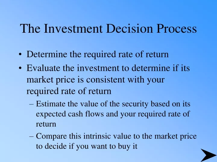
The Investment Decision Process • Determine the required rate of return • Evaluate the investment to determine if its market price is consistent with your required rate of return • Estimate the value of the security based on its expected cash flows and your required rate of return • Compare this intrinsic value to the market price to decide if you want to buy it
Valuation Process • Two approaches • 1. Top-down, three-step approach • 2. Bottom-up, stock valuation, stock picking approach • The difference between the two approaches is the perceived importance of economic and industry influence on individual firms and stocks
Theory of Valuation • The value of an asset is the present value of its expected returns • You expect an asset to provide a stream of returns while you own it
Theory of Valuation • To convert this stream of returns to a value for the security, you must discount this stream at your required rate of return • This requires estimates of: • The stream of expected returns, and • The required rate of return on the investment
Stream of Expected Returns • Form of returns • Earnings • Cash flows • Dividends • Interest payments • Capital gains (increases in value) • Time pattern and growth rate of returns
Required Rate of Return • Determined by • 1. Economy’s risk-free rate of return, plus • 2. Expected rate of inflation during the holding period, plus • 3. Risk premium determined by the uncertainty of returns
Investment Decision Process: A Comparison of Estimated Values and Market Prices If Estimated Value > Market Price, Buy If Estimated Value < Market Price, Don’t Buy
Approaches to the Valuation of Common Stock Two approaches have developed 1. Discounted cash-flow valuation • Present value of some measure of cash flow, including dividends, operating cash flow, and free cash flow 2. Relative valuation technique • Value estimated based on its price relative to significant variables, such as earnings, cash flow, book value, or sales
Approaches to the Valuation of Common Stock The discounted cash flow approaches are dependent on some factors, namely: • The rate of growth and the duration of growth of the cash flows • The estimate of the discount rate
Why and When to Use the Discounted Cash Flow Valuation Approach • The measure of cash flow used • Dividends • Cost of equity as the discount rate • Operating cash flow • Weighted Average Cost of Capital (WACC) • Free cash flow to equity • Cost of equity • Dependent on growth rates and discount rate
Why and When to Use the Relative Valuation Techniques • Provides information about how the market is currently valuing stocks • aggregate market • alternative industries • individual stocks within industries • No guidance as to whether valuations are appropriate • best used when have comparable entities • aggregate market is not at a valuation extreme
Discounted Cash-Flow Valuation Techniques Where: Vj = value of stock j n = life of the asset CFt = cash flow in period t k = the discount rate that is equal to the investor’s required rate of return for asset j, which is determined by the uncertainty (risk) of the stock’s cash flows
Valuation Approaches and Specific Techniques Approaches to Equity Valuation Figure 13.2 Discounted Cash Flow Techniques Relative Valuation Techniques • Price/Earnings Ratio (PE) • Price/Cash flow ratio (P/CF) • Price/Book Value Ratio (P/BV) • Price/Sales Ratio (P/S) • Present Value of Dividends (DDM) • Present Value of Operating Cash Flow • Present Value of Free Cash Flow
The Dividend Discount Model (DDM) The value of a share of common stock is the present value of all future dividends Where: Vj = value of common stock j Dt = dividend during time period t k = required rate of return on stock j
The Dividend Discount Model (DDM) If the stock is not held for an infinite period, a sale at the end of year 2 would imply:
The Dividend Discount Model (DDM) If the stock is not held for an infinite period, a sale at the end of year 2 would imply: Selling price at the end of year two is the value of all remaining dividend payments, which is simply an extension of the original equation
The Dividend Discount Model (DDM) Stocks with no dividends are expected to start paying dividends at some point
The Dividend Discount Model (DDM) Stocks with no dividends are expected to start paying dividends at some point, say year three...
The Dividend Discount Model (DDM) Stocks with no dividends are expected to start paying dividends at some point, say year three... Where: D1 = 0 D2 = 0
The Dividend Discount Model (DDM) Infinite period model assumes a constant growth rate for estimating future dividends
The Dividend Discount Model (DDM) Infinite period model assumes a constant growth rate for estimating future dividends Where: Vj = value of stock j D0 = dividend payment in the current period g = the constant growth rate of dividends k = required rate of return on stock j n = the number of periods, which we assume to be infinite
The Dividend Discount Model (DDM) Infinite period model assumes a constant growth rate for estimating future dividends This can be reduced to: 1. Estimate the required rate of return (k) 2. Estimate the dividend growth rate (g)
Infinite Period DDM and Growth Companies Assumptions of DDM: 1. Dividends grow at a constant rate 2. The constant growth rate will continue for an infinite period 3. The required rate of return (k) is greater than the infinite growth rate (g)
Infinite Period DDM and Growth Companies Growth companies have opportunities to earn return on investments greater than their required rates of return To exploit these opportunities, these firms generally retain a high percentage of earnings for reinvestment, and their earnings grow faster than those of a typical firm This is inconsistent with the infinite period DDM assumptions
Infinite Period DDM and Growth Companies The infinite period DDM assumes constant growth for an infinite period, but abnormally high growth usually cannot be maintained indefinitely Risk and growth are not necessarily related Temporary conditions of high growth cannot be valued using DDM
Valuation with Temporary Supernormal Growth Combine the models to evaluate the years of supernormal growth and then use DDM to compute the remaining years at a sustainable rate For example: With a 14 percent required rate of return and dividend growth of:
Valuation with Temporary Supernormal Growth Dividend Year Growth Rate 1-3: 25% 4-6: 20% 7-9: 15% 10 on: 9%
Valuation with Temporary Supernormal Growth The value equation becomes
Computation of Value for Stock of Company with Temporary Supernormal Growth Exhibit 11.3
Present Value of Operating Free Cash Flows • Derive the value of the total firm by discounting the total operating cash flows prior to the payment of interest to the debt-holders • Then subtract the value of debt to arrive at an estimate of the value of the equity
Present Value of Operating Free Cash Flows Where: Vj = value of firm j n = number of periods assumed to be infinite OCFt = the firms operating free cash flow in period t WACC = firm j’s weighted average cost of capital
Present Value of Operating Free Cash Flows Similar to DDM, this model can be used to estimate an infinite period Where growth has matured to a stable rate, the adaptation is Where: OCF1=operating free cash flow in period 1 gOCF = long-term constant growth of operating free cash flow
Present Value of Operating Free Cash Flows • Assuming several different rates of growth for OCF, these estimates can be divided into stages as with the supernormal dividend growth model • Estimate the rate of growth and the duration of growth for each period
Present Value of Free Cash Flows to Equity • “Free” cash flows to equity are derived after operating cash flows have been adjusted for debt payments (interest and principle) • The discount rate used is the firm’s cost of equity (k) rather than WACC
Present Value of Free Cash Flows to Equity Where: Vj = Value of the stock of firm j n = number of periods assumed to be infinite FCFt = the firm’s free cash flow in period t K j =the cost of equity
Relative Valuation Techniques • Value can be determined by comparing to similar stocks based on relative ratios • Relevant variables include earnings, cash flow, book value, and sales • The most popular relative valuation technique is based on price to earnings
Earnings Multiplier Model • This values the stock based on expected annual earnings • The price earnings (P/E) ratio, or Earnings Multiplier
Earnings Multiplier Model The infinite-period dividend discount model indicates the variables that should determine the value of the P/E ratio
Earnings Multiplier Model The infinite-period dividend discount model indicates the variables that should determine the value of the P/E ratio Dividing both sides by expected earnings during the next 12 months (E1)
Earnings Multiplier Model Thus, the P/E ratio is determined by 1. Expected dividend payout ratio 2. Required rate of return on the stock (k) 3. Expected growth rate of dividends (g)
Earnings Multiplier Model As an example, assume: • Dividend payout = 50% • Required return = 12% • Expected growth = 8% • D/E = .50; k = .12; g=.08
Earnings Multiplier Model As an example, assume: • Dividend payout = 50% • Required return = 12% • Expected growth = 8% • D/E = .50; k = .12; g=.08
Earnings Multiplier Model Given current earnings of $2.00 and growth of 9% You would expect E1 to be $2.18 D/E = .50; k=.12; g=.09 P/E = 16.7 V = 16.7 x $2.18 = $36.41 Compare this estimated value to market price to decide if you should invest in it
Estimating the Inputs: The Required Rate of Return and The Expected Growth Rate of Valuation Variables Valuation procedure is the same for securities around the world, but the required rate of return (k) and expected growth rate of earnings and other valuation variables (g) such as book value, cash flow, and dividends differ among countries
Required Rate of Return (k) The investor’s required rate of return must be estimated regardless of the approach selected or technique applied • This will be used as the discount rate and also affects relative-valuation • This is not used for present value of free cash flow which uses the required rate of return on equity (K) • It is also not used in present value of operating cash flow which uses WACC
Required Rate of Return (k) Three factors influence an investor’s required rate of return: • The economy’s real risk-free rate (RRFR) • The expected rate of inflation (I) • A risk premium (RP)
Expected Growth Rate of Dividends • Determined by • the growth of earnings • the proportion of earnings paid in dividends • In the short run, dividends can grow at a different rate than earnings due to changes in the payout ratio • Earnings growth is also affected by compounding of earnings retention g = (Retention Rate) x (Return on Equity) = b x ROE
Valuation of Alternative Investments • Valuation of Bonds is relatively easy because the size and time pattern of cash flows from the bond over its life are known 1. Interest payments are made usually every six months equal to one-half the coupon rate times the face value of the bond 2. The principal is repaid on the bond’s maturity date
Valuation of Bonds • Example: in 2002, a $10,000 bond due in 2017 with 10% coupon • Discount these payments at the investor’s required rate of return (if the risk-free rate is 9% and the investor requires a risk premium of 1%, then the required rate of return would be 10%)
Valuation of Bonds Present value of the interest payments is an annuity for thirty periods at one-half the required rate of return: $500 x 15.3725 = $7,686 The present value of the principal is similarly discounted: $10,000 x .2314 = $2,314 Total value of bond at 10 percent = $10,000