Download
1 / 45
450 likes | 583 Views
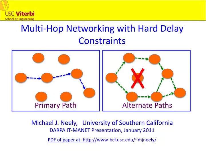
Multi-Hop Networking with Hard Delay Constraints. B. Primary Path. Alternate Paths. Michael J. Neely, University of Southern California DARPA IT-MANET Presentation, January 2011 PDF of paper at: http:// www- bcf.usc.edu/~mjneely /. IT-MANET Topics:.

E N D
Multi-Hop Networking with Hard Delay Constraints B Primary Path Alternate Paths Michael J. Neely, University of Southern California DARPA IT-MANET Presentation, January 2011 PDF of paper at: http://www-bcf.usc.edu/~mjneely/
IT-MANET Topics: • Non-Equilibrium Networking for MANETS • Delay Guarantees • Optimization of Throughput-Utility • M. J. Neely, “Opportunistic Scheduling with Worst Case Delay Guarantees • in Single and Multi-Hop Networks,” Proc. IEEE INFOCOM 2011. • This work builds on: • i) “Universal Scheduling” (Neely, Proc. IEEE CDC 2010) • ARL CTA Task. • Social Networks extensions: • M. J. Neely, L. Golubchik, “Utility Optimization for Dynamic Peer-to-Peer • Networks with Tit-for-Tat Constraints,” Proc. IEEE INFOCOM 2011. • ii) “Hop Count Limited Networking” (IT-MANET, PI Shakkottai) • L. Ying, S. Shakkottai, A. Reddy, “On Combining Shortest Path And Back-pressure • Routing over Multihop Wireless Networks,” Proc. IEEE INFOCOM 2009.
Want to optimally react to unexpected events. Example 1: Failure at Node B C A B D C A B D Primary Path Alternate Paths
Example 2: Opportunity via Mobility mobile node Primary Path C A B D
Example 2: Opportunity via Mobility mobile node Primary Path C A B D
Example 2: Opportunity via Mobility mobile node Primary Path C A B D
Example 2: Opportunity via Mobility mobile node Primary Path C A B D
Example 2: Opportunity via Mobility mobile node Primary Path C A B D
Example 2: Opportunity via Mobility mobile node Primary Path C A B D
Example 2: Opportunity via Mobility mobile node Primary Path C A B D
Example 2: Opportunity via Mobility mobile node Primary Path C A B D
Example 2: Opportunity via Mobility mobile node Primary Path C A B D
Example 2: Opportunity via Mobility mobile node Primary Path C A B D
Example 2: Opportunity via Mobility mobile node Primary Path C A B D
Example 2: Opportunity via Mobility mobile node Primary Path C A B D
Assumptions and Main Questions: • Assumptions: • Arbitrary mobility, traffic, channels. • Little or no probability models known in advance. • Any sample path is possible (non-ergodic). • Future is unknown. • Questions: • Can we develop math for non-equilibrium networks? • Can we optimize without knowing the future? • Can we make worst-case delay guarantees?
Main Results: • We use a backpressure/max-weight algorithm • that does not know future. • Design a novel “ε-persistent service” virtual queue • for delay guarantees. • Use “T-Slot Lookahead Utility” defined by an “ideal” • alg. that has perfect knowledge of the future up to T slots. • For any T, our algorithm can achieve utility that is • arbitrarily close to the T-slot Lookahead utility, • with tradeoff in worst case delay.
Problem Formulation: • Timeslotted system, slots t = {0, 1, 2, …}. • N node MANET. • M data flows (each with source-destination). • No pre-specified routes (we learn them).
Problem Formulation: • Timeslotted system, slots t = {0, 1, 2, …}. • N node MANET. • M data flows (each with source-destination). • No pre-specified routes (we learn them). 4 Nodes: N = 8 5 8 1 2 3 7 6
Problem Formulation: • Timeslotted system, slots t = {0, 1, 2, …}. • N node MANET. • M data flows (each with source-destination). • No pre-specified routes (we learn them). 4 Nodes: N = 8 Flows: M = 3 5 8 1 2 3 7 6
Problem Formulation: • Timeslotted system, slots t = {0, 1, 2, …}. • N node MANET. • M data flows (each with source-destination). • No pre-specified routes (we learn them). 4 • Nodes: N = 8 • Flows: M = 3 • Flow 1: 13 5 1 8 1 2 3 7 6
Problem Formulation: • Timeslotted system, slots t = {0, 1, 2, …}. • N node MANET. • M data flows (each with source-destination). • No pre-specified routes (we learn them). 4 • Nodes: N = 8 • Flows: M = 3 • Flow 1: 13 • Flow 2: 73 5 1 8 1 2 3 7 6 2
Problem Formulation: • Timeslotted system, slots t = {0, 1, 2, …}. • N node MANET. • M data flows (each with source-destination). • No pre-specified routes (we learn them). 3 4 • Nodes: N = 8 • Flows: M = 3 • Flow 1: 13 • Flow 2: 73 • Flow 3: 56 5 1 8 1 2 3 7 6 2
Problem Formulation: • Timeslotted system, slots t = {0, 1, 2, …}. • N node MANET. • M data flows (each with source-destination). • No pre-specified routes (we learn them). 3 4 • Nodes: N = 8 • Flows: M = 3 • Flow 1: 13 • Flow 2: 73 • Flow 3: 56 5 1 8 1 2 3 7 6 2
State Information and Network Decisions: • S(t) = “Topology State” observed on slot t. • (μij(c)(t)) = Transmission Decisions (in set Γ(S(t)) Sij(t) Sik(t)
How to enforce delay guarantees? • (1) Allow Packet Dropping at Source Flow Control: • (2) Allow Packet Dropping at in-Network Queues: Rm(t) Source node m Am(t) Qj(t) arrivalsj(t) μj(t) Dj(t) Maximize: ∑ gm(rm – dm) Subject to: Net. Stability Maximize: ∑ [gm(rm) – νmdm] Subject to: Net. Stability rm = time avg admission rate of flow m dm = time avg packet drops of flow m This transformation separates out the variables, and is useful for distributed implementation.
How to enforce delay guarantees? • (1) Allow Packet Dropping at Source Flow Control: • (2) Allow Packet Dropping at in-Network Queues: Rm(t) Source node m Am(t) Qj(t) arrivalsj(t) μj(t) Dj(t) Maximize: ∑ gm(rm – dm) Subject to: Net. Stability Maximize: ∑ [gm(γm) – νmdm] Subject to: rm ≥ γm Net. Stability rm = time avg admission rate of flow m dm = time avg packet drops of flow m This transformation turns a maximization of a function of a time average into a maximization of a pure time average.
How to enforce delay guarantees? • (3) Use New Virtual Queue for ε-Persistent Service: • Theorem: If Qj(t) ≤ Qmax, Zj(t) ≤ Zmax, then: • Worst Case Delay in Node j ≤ (Qmax + Zmax)/ε Actual Queue: Qj(t) arrivalsj(t) μj(t)+Dj(t) Zj(t) Virtual Queue: ε 1{Qj(t)>0} μj(t)+Dj(t) a(t) Q(t) ≤ Qmax t t+MaxDelay
Utility Maximization with T-Slot Lookahead: • Segment timeline into T-slot frames. • φopt[r] = optimal sum utility over frame r, • assuming future is known in frame! Frame 0 Frame 2 Frame 1 • Value of φopt[r] can be written as a non-linear • program (assuming future arrivals, channels, • and topology states are known)…
Analytical Approach: • Lyapunov Function for queues: L(Q(t)) = ∑ [Qi(t)2 +Zi(t)2 + Yi(t)2] • New sample path “T-slot” Lyapunov Drift: • ΔT(t) = L(Q(t+T)) – L(Q(t)) • Every slot “greedily” minimize 1-slot drift-plus-penalty: • Δ1(t) + V xPenalty(t) , Penalty(t) = -φ(γ(t))+νmDm(t) • Results in a joint backpressure, flow control, packet dropping alg with modified backpressure weights: Qj(t) + Zj(t)1{Qj(t)>0}
Performance Result • Theorem: Arbitrary Traffic, Mobility. For any R>0, T>0: • (ii) Worst Case Queue Delay = B3V/ε • B1, Β2 , Β3 are known constants. • V = “knob” to turn to affect the tradeoff • R = Running Time (number of T-slot frames) Achieved Utility over RT slots ≥ (1/R)∑r=0φopt[r]– “Fudge Factor” R-1 B1T + B2V (i) “Fudge Factor” = V RT O(1/V), O(V) utility-backlog tradeoff when time horizon R infinity
Conclusions: • Arbitrary Traffic, Mobility (can be “non-ergodic”). • New Math for “Non-Equilibrium” Networking. • O(V), O(1/V) tradeoff between worst case queue delay and network utility. • Easily extends to worst-case end-to-end delay via: • (i) Restrict routing paths to H hops. • (ii) Use PI Shakkottai result on H-hop limited Queueing. • New Book Advertisement: • M. J. Neely, Stochastic Network Optimization with Application to Communication and Queueing Systems. Morgan & Claypool, 2010. • PDF available from “Synthesis Lecture Series” (on digital library), link • on Neely homepage (for PDF and/or order form for hardcopy)
Extra Detail Slides: • Network Transmission Model • Some Simulations for “Universal Scheduling” in the presence of non-ergodic traffic and jamming.
Network Queueing: a b a • Each node keeps queues for each separate commodity (“commodity” = “destination”). • For commodity c (say, green commodity): • Qa(c)(t+1) = Qa(c)(t) – Transmit out • + Endogenous Arrivals + Exogenous Arrivals
Example Mobile Network: • Five Mobility Groups: • 10 nodes Group 1 (upper left) • 10 nodes Group 2 (upper right) • 10 nodes Group 3 (lower right) • 10 nodes Group 4 (lower left) • 1 node Group 5 D1 S1 S2 Group 1 nodes: Random Walk on Upper Left Region
Example Mobile Network: • Five Mobility Groups: • 10 nodes Group 1 (upper left) • 10 nodes Group 2 (upper right) • 10 nodes Group 3 (lower right) • 10 nodes Group 4 (lower left) • 1 node Group 5 D1 S1 S2 Group 2 nodes: Random Walk on Upper Right Region
Example Mobile Network: • Five Mobility Groups: • 10 nodes Group 1 (upper left) • 10 nodes Group 2 (upper right) • 10 nodes Group 3 (lower right) • 10 nodes Group 4 (lower left) • 1 node Group 5 D1 S1 S2 Group 3 nodes: Random Walk on Lower Right Region
Example Mobile Network: • Five Mobility Groups: • 10 nodes Group 1 (upper left) • 10 nodes Group 2 (upper right) • 10 nodes Group 3 (lower right) • 10 nodes Group 4 (lower left) • 1 node Group 5 D1 S1 S2 Group 4 nodes: Random Walk on Lower Left Region
Example Mobile Network: • Five Mobility Groups: • 10 nodes Group 1 (upper left) • 10 nodes Group 2 (upper right) • 10 nodes Group 3 (lower right) • 10 nodes Group 4 (lower left) • 1 node Group 5 D1 S1 S2 Group 5 node: Periodically cycles about the clockwise orbit
Example Mobile Network: Sim. 1– Change Social Contacts Backlog Bound for D1 in a sample RED node D1 S1 Backlog Bound for S1 in a sample RED node S2 • Social Contacts: • Source 1: S1D1 (constant rate = 0.07 packets/slot) • Source 2: S2 S1 (for first half of simulation) • S2 D1 (for second half of simulation) • Goal: Maximize Throughput of Source 2 subject to stability • Use V=10, so guarantee no more that 11 source 2 packets • in any queue!
Example Mobile Network: Sim. 1– Change Social Contacts Moving Average thruput:S2D1 D1 S1 Moving Average thruput:S2S1 S2 • Social Contacts: • Source 1: S1D1 (constant rate = 0.07 packets/slot) • Source 2: S2 S1 (for first half of simulation) • S2 D1 (for second half of simulation) • Goal: Maximize Throughput of Source 2 subject to stability • Use V=10, so guarantee no more that 11 source 2 packets • in any queue!
Example Mobile Network: Sim. 1– Change Social Contacts Moving Average thruput:S2D1 D1 S1 Moving Average thruput:S2S1 S2 • Overall Performance is Seamless: • Backlog no more than 11 packets in any queue for Source 1 data • Backlog no more than 15 packets in any queue for Source 2 data • Overall Thruput of Source 2 is maintained at near-optimal over the • change, even though the routes must fundamentally change!
Example Mobile Network: Sim. 2– Intermittent Jamming JAM! JAM! Time D1 S1 S2 • Social Contacts: • Source 1: S1D1 (constant rate = 0.07 packets/slot) • Source 2: S2 S1 (Goal to maximize its throughput) • Intermittent Interference during 2 intervals of the simulation • That completely cut interaction between the groups 1-4. • Can only use the cyclic mobile node at these times! • Max Thruput of Source 2 during interference ~= 0.03.
Example Mobile Network: Sim. 2– Intermittent Jamming D1 JAM! S1 JAM! Time S2 • Social Contacts: • Source 1: S1D1 (constant rate = 0.07 packets/slot) • Source 2: S2 S1 (Goal to maximize its throughput) • Intermittent Interference during 2 intervals of the simulation • That completely cut interaction between the groups 1-4. • Can only use the cyclic mobile node at these times! • Max Thruput of Source 2 during interference ~= 0.03.
Conclusion Slide: Backlog Bound for D1 in a sample RED node D1 S1 Backlog Bound for S1 in a sample RED node Moving Average Thruput of Source 2 S2 • Overall Seamless Operation • Throughput During Jamming goes down, • but is close to optimal value of 0.03. • Fudge Factor = BT/V + CV/RT • Worst Case Queue Backlog = O(V) • Framework useful for stock market trading! (Thursday @ 10:20am)