Download
1 / 23
230 likes | 356 Views
Simulating Adiabatic Parcel Rise. Presentation by Anna Merrifield, Sarah Shackleton and Jeff Sussman. Buoyancy Force. Relationship of parcel density to atmospheric density At a given pressure, density is determined by Temperature. Buoyancy Force.

E N D
Simulating Adiabatic Parcel Rise Presentation by Anna Merrifield, Sarah Shackleton and Jeff Sussman
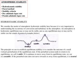
Buoyancy Force • Relationship of parcel density to atmospheric density • At a given pressure, density is determined by Temperature
Buoyancy Force • If the parcel is less dense (warmer) than the atmosphere it will rise adiabatically and cool • T’ > Tenv • If parcel is more dense (cooler) than the environment it will sink adiabatically and warm • T’ < Tenv
Real World Examples of Parcel Rise • Cloud formation • If the environment is stable, clouds that form will be shallow (stratus clouds) • In an unstable environment, vertical motion occurs, cumulus and cumulonimbus form • Thunderstorms/Tornadoes • With enough parcel rise, thunderstorms can form
CAPE • Convective available potential energy • Amount of potential energy available for parcel rise • Important for thunderstorm growth/formation
Parcel Method • The parcel does not mix with the surrounding environment • The parcel does not disturb its environment • The pressure of the parcel adjusts instantaneously to its environment • The parcel moves isentropically
The Model • Obtain the data from Figure 7.2 using DataThief • Determine Z(P,T) • Model Parcel Temperature assuming: • Dry adiabatic rise to LCL • Saturated adiabatic rise to LNB • “Moist” adiabatic rise above the LNB • Model Parcel Temperature assuming: • Dry adiabatic rise to LCL • Saturated adiabatic rise while entraining dry air to LNB • “Moist” adiabatic rise above the LNB • Sensitivity analysis: find lapse rates that reproduce the model
1. Obtaining the Data The plot lines were redrawn in color to allow for effective tracing. Markers indicate the axes and the beginning, color, and end of the line we want to trace. After the line is traced, the program picks points on the line and the data can be output and read into Matlab.
1. Problems with DataThief Solution: Rather than throwing out points (they aren’t “bad”, we determined Z using a linear least-squares fit to 3 regions of constant lapse rate
2. Determining Z(P,T) Γ = .64 K/Km Γ = 3.6 K/Km Regions of ~Constant Lapse Rate Γ = 6.5 K/Km
Dry & Saturated Adiabatic Lapse Rates • Dry lapse rate: assumptions – ideal gas, atmosphere is in hydrostatic equilibrium, no water vapor • Saturated lapse rate: assumptions – no loss of water through precipitation, only liquid and vapor phases, system at chemical equilibrium, and heat capacities of liquid and water vapor are negligible, parcel has reached 100% relative humidity
Modeling Saturated Adiabatic Rise 1. Initialize esat(1), Tparcel (1)
The Second Model • Entrainment: The mixing of the rising air parcel with the surrounding environment • Entrainment rate: 1/m dm/dz • Assumptions: entrainment of dry air, constant entrainment rate, isotropic entrainment
Discussion • Lack of CAPE in all models • Limitations of the simplified model • Parcel movement adiabatic and reversible (no precipitation) • Entrainment of dry air • Sounding given as lnP versus T, not given with altitude which then needed to be derived using assumption of constant lapse rate atmosphere in three regions • DataThief does not give monotonically increasing data points
5. Reproduction of Figure 7.2 LNB LCL
CAPE example with entrainment Image from NWS from Amarillo, TX, July 22,2013
Conclusions and Further Work • Failure to reproduce plot using simplified governing assumptions of adiabatic parcel rise • Further work using soundings from a database http://weather.uwyo.edu/upperair/sounding.html