Download
1 / 52
530 likes | 744 Views
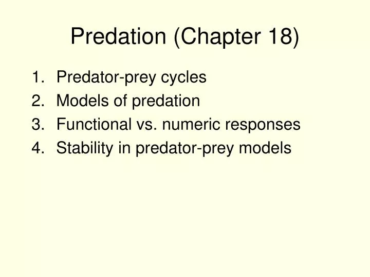
Predation (Chapter 18). Predator-prey cycles Models of predation Functional vs. numeric responses Stability in predator-prey models. Two big themes:. Predators can limit prey populations. This keeps populations below K .

E N D
Predation (Chapter 18) • Predator-prey cycles • Models of predation • Functional vs. numeric responses • Stability in predator-prey models
Two big themes: • Predators can limit prey populations. This keeps populations below K.
Predator and prey populations increase and decrease in regular cycles.
A verbal model of predator-prey cycles: • Predators eat prey and reduce their numbers • Predators go hungry and decline in number • With fewer predators, prey survive better and increase • Increasing prey populations allow predators to increase And repeat…
The Lotka-Volterra Model: Assumptions • Prey grow exponentially in the absence of predators. • Predation is directly proportional to the product of prey and predator abundances (random encounters). • Predator populations grow based on the number of prey. Death rates are independent of prey abundance.
R = prey population size (“resource”) P = predator population size r = exponential growth rate of the prey c = capture efficiency of the predators
removal of prey by predators rate of change in the prey population intrinsic growth rate of the prey
For the predators: a = efficiency with which prey are converted into predators d = death rate of predators death rate of predators rate of change in the predator population conversion of prey into new predators
Prey population reaches equilibrium when dR/dt = 0 • equilibrium – state of balance between opposing forces • populations at equilibrium do not change • Prey population stabilizes based on the size of the predator population
Predator population reaches equilibriumwhen dP/dt = 0 • Predator population stabilizes based on the size of the prey population
Isocline – a line along which populations will not change over time. • Predator numbers will stay constant if R = d/ac • Prey numbers will stay constant if P = r/c.
Predators are stable when: Prey are stable when: Number of Predators (P) Number of prey (R)
Prey are stable when: Prey Isocline Number of Predators (P) r/c d/ac Number of prey (R)
Predators are stable when: Predator isocline Number of Predators (P) d/ac Number of prey (R)
equilibrium Number of Predators (P) r/c d/ac Number of prey (R)
Predation (Chapter 18) • Finish Lotka-Volterra model • Functional vs. numeric responses • Stability in predator-prey cycles
Number of predators depends on the prey population. Predator isocline Number of Predators (P) Predators decrease Predators increase d/ac Number of prey (R)
Number of prey depends on the predator population. Prey decrease Prey Isocline Number of Predators (P) r/c Prey increase d/ac Number of prey (R)
Changing the number of prey can cause 2 types of responses: Functional response – relationship between an individual predator’s food consumption and the density of prey Numeric response – change in the population of predators in response to prey availability
Lotka-Volterra: prey are consumed in direct proportion to their availability (cRP term) • known as Type I functional response • predators never satiate! • no limit on the growth rate of predators!
Type II functional response – consumption rate increases at first, but eventually predators satiate (upper limit on consumption rate)
Type III functional response – consumption rate is low at low prey densities, increases, and then reaches an upper limit
Why type III functional response? • at low densities, prey may be able to hide, but at higher densities hiding spaces fill up • predators may be more efficient at capturing more common prey • predators may switch prey species as they become more/less abundant
Numeric response comes from • Population growth • (though most predator populations grow slowly) • Immigration • predator populations may be attracted to prey outbreaks
Predator-prey cycles can be unstable • efficient predators can drive prey to extinction • if the population moves away from the equilibrium, there is no force pulling the populations back to equilibrium • eventually random oscillations will drive one or both species to extinction
Factors promoting stability in predator-prey relationships • Inefficient predators (prey escaping) • less efficient predators (lower c) allow more prey to survive • more living prey support more predators • Outside factors limit populations • higher d for predators • lower r for prey
Alternative food sources for the predator • less pressure on prey populations • Refuges from predation at low prey densities • prevents prey populations from falling too low • Rapid numeric response of predators to changes in prey population
Huffaker’s experiment on predator-prey coexistence • 2 mite species, predator and prey
Initial experiments – predators drove prey extinct then went extinct themselves • Adding barriers to dispersal allowed predators and prey to coexist.
Prey population outbreaks Population growth curve for logistic population growth Per capita population growth rate ro K Density of prey population
Type III functional response curve for predators Per capita death rate K Density of prey population
Point A – stable equilibrium; population increases below A and decreases above A A
Unstable equilibrium – equilibrium point from which a population will move to a new, different equilibrium if disturbed
Point B – unstable equilibrium; below B, predation reduces population to A; above B, predators are less efficient, so population grows to C B
Between B & C – predators are less efficient, prey increase up to C B
Predator-prey systems can have multiple stable states • Reducing the number of predators can lead to an outbreak of prey