Download
1 / 25
250 likes | 269 Views
Lecture 2: Measuring Performance/Cost/Power. Today’s topics: (Sections 1.6, 1.4, 1.7, 1.8) Quantitative principles of computer design Measuring cost Real industrial examples. Summarizing Performance. Recall discussion on AM versus GM GM: does not require a reference machine, but does

E N D
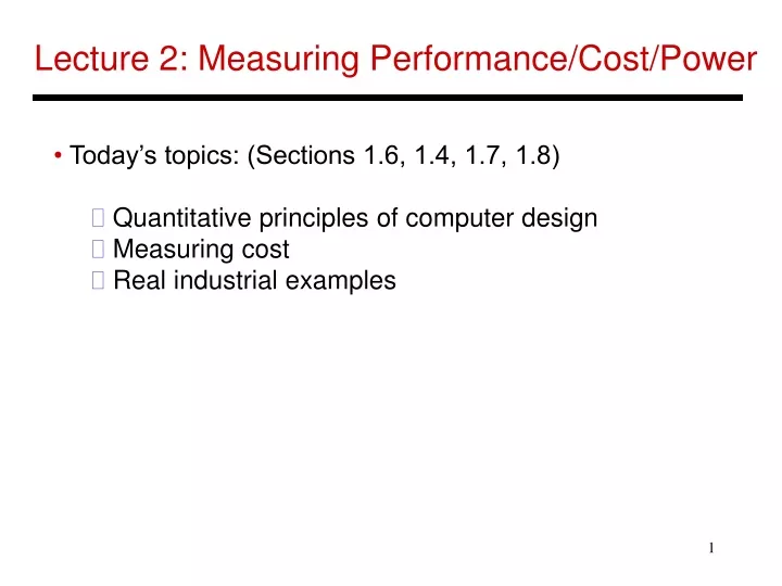
Lecture 2: Measuring Performance/Cost/Power • Today’s topics: (Sections 1.6, 1.4, 1.7, 1.8) • Quantitative principles of computer design • Measuring cost • Real industrial examples
Summarizing Performance • Recall discussion on AM versus GM • GM: does not require a reference machine, but does • not predict performance very well • So we multiplied execution times and determined that sys-A is 1.2x faster…but on what workload? • AM: does predict performance for a specific workload, • but that workload was determined by executing • programs on a reference machine • Every year or so, the reference machine will have to be updated
Example • We fixed a reference machine X and ran 4 programs • A, B, C, D on it such that each program ran for 1 second • The exact same workload (the four programs execute • the same number of instructions that they did on • machine X) is run on a new machine Y and the • execution times for each program are 0.8, 1.1, 0.5, 2 • With AM of normalized execution times, we can conclude • that Y is 1.1 times slower than X – perhaps, not for all • workloads, but definitely for one specific workload (where • all programs run on the ref-machine for an equal #cycles) • With GM, you may find inconsistencies
GM Example • Computer-A Computer-B Computer-C • P1 1 sec 10 secs 20 secs • P2 1000 secs 100 secs 20 secs • Conclusion with GMs: (i) A=B • (ii) C is ~1.6 times faster • For (i) to be true, P1 must occur 100 times for every • occurrence of P2 • With the above assumption, (ii) is no longer true • Hence, GM can lead to inconsistencies
CPU Performance Equation • CPU time = clock cycle time x cycles per instruction x • number of instructions • Influencing factors for each: • clock cycle time: technology and organization • CPI: organization and instruction set design • instruction count: instruction set design and compiler • CPI (cycles per instruction) or IPC (instructions per cycle) • can not be accurately estimated analytically
Measuring System CPI • Assume that an architectural innovation only affects CPI • For 3 programs, base CPIs: 1.2, 1.8, 2.5 • CPIs for proposed model: 1.4, 1.9, 2.3 • What is the best way to summarize performance with a • single number? AM, HM, or GM of CPIs?
Example • AM of CPI for base case = 1.2 cyc + 1.8 cyc + 2.5 cyc • instr instr instr • 5.5 cycles is execution time if each program ran for • one instruction – therefore, AM of CPI defines a • workload where every program runs for an equal #instrs • HM of CPI = 1 / AM of IPC ; defines a workload where • every program runs for an equal number of cycles • GM of CPI: warm fuzzy number, not necessarily • representing any workload
Amdahl’s Law • Architecture design is very bottleneck-driven – make the • common case fast, do not waste resources on a component • that has little impact on overall performance/power • Amdahl’s Law: performance improvements through an • enhancement is limited by the fraction of time the • enhancement comes into play • Example: a web server spends 40% of time in the CPU • and 60% of time doing I/O – a new processor that is ten • times faster results in a 36% reduction in execution time • (speedup of 1.56) – Amdahl’s Law states that maximum • execution time reduction is 40% (max speedup of 1.66)
Principle of Locality • Most programs are predictable in terms of instructions • executed and data accessed • The 90-10 Rule: a program spends 90% of its execution • time in only 10% of the code • Temporal locality: a program will shortly re-visit X • Spatial locality: a program will shortly visit X+1
Exploit Parallelism • Most operations do not depend on each other – hence, • execute them in parallel • At the circuit level, simultaneously access multiple ways • of a set-associative cache • At the organization level, execute multiple instructions at • the same time • At the system level, execute a different program while one • is waiting on I/O
Factors Determining Cost • Cost: amount spent by manufacturer to produce a finished • good • High volume faster learning curve, increased • manufacturing efficiency (10% lower cost if volume doubles), • lower R&D cost per produced item • Commodities: identical products sold by many vendors in • large volumes (keyboards, DRAMs) – low cost because of • high volume and competition among suppliers
Wafers and Dies An entire wafer is produced and chopped into dies that undergo testing and packaging
Integrated Circuit Cost • Cost of an integrated circuit = • (cost of die + cost of packaging and testing) / final test yield • Cost of die = cost of wafer / (dies per wafer x die yield) • Dies/wafer = wafer area / die area - p wafer diam / die diag • Die yield = wafer yield x (1 + (defect rate x die area) / a) -a • Thus, die yield depends on die area and complexity • arising from multiple manufacturing steps (a ~ 4.0)
Integrated Circuit Cost Examples • A 30 cm diameter wafer cost $5-6K in 2001 • Such a wafer yields about 366 good 1 cm2 dies and 1014 • good 0.49 cm2 dies (note the effect of area and yield) • Die sizes: Alpha 21264 1.15 cm2 , Itanium 3.0 cm2 , • embedded processors are between 0.1 – 0.25 cm2
Cost and Price • A $1000 increase in cost may result in a $3000 increase • in price – hence, important to understand the relationship • The relationship is complex – for example, a company may • underprice a product that has heavy competition and • overprice a product that has no competition
Computing Price • Component costs: developing wafers, testing, packaging • Direct costs: 10-30% of component costs: labor, warranty • Gross margin (indirect costs): 10-45% of sum of these • three (average selling price): R&D, marketing, sales, • building rental, profits • Retail mark-up: sum of all the above gives list price • Low-end PCs may have low gross margins – low R&D, • low cost for sales, low profits • R&D costs are only 4-12%
Desktop Prices All systems have similar configurations – price variations due to expandability, expensive disks/memory/processor/OS, commoditization
Server Performance Using the OLTP benchmark TPC-C
Embedded Prices • Does not include the prices and power of support chips • High variance in functionality, price, performance, power • The IBM and AMD processors are used in network switches • and laptops, the NEC VR 5432 is used in laser printers, the • NEC VR 4122 is used in PDAs
Title • Bullet