Fall 2013 CMU CS 15-855 Computational Complexity

1. Fall 2013 CMU CS 15-855Computational Complexity Introduction Lecture 1

2. Complexity Theory Classify problems according to the computational resources required • running time • storage space • parallelism • randomness • rounds of interaction, communication, others… Attempt to answer: what is computationally feasible with limited resources?

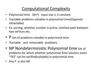
3. The central questions • Is finding a solution as easy as recognizing one? P = NP? • Is every efficient sequential algorithm parallelizable? P = NC? • Can every efficient algorithm be converted into one that uses a tinyamount of memory? P = L? • Are there small Boolean circuits for all problems that require exponential running time? EXP  P/poly? • Can every efficient randomized algorithm be converted into a deterministic algorithm one? P = BPP?

4. Languages • Let ∑be any finite alphabet. • L µ∑* • L is a language. • The decision problem corresponding to L is the function: f:∑*! {yes, no} deciding membership in L, i.e., {x | f(x)=‘yes} • Examples: • set of strings encoding satisfiable formulas • set of strings that encode pairs (n,k) for which n has factor < k

5. Historical:One Tape Turing Machine . . . a b a b infinite tape finite control read/write head

6. Turing Machines • Q finite set of states • ∑ alphabet including blank: “_” • qstart, qaccept, qrejectin Q • δ : Q x ∑! Q x ∑ x {L, R, -} transition fn. • input written on tape, head on 1st square, state qstart • sequence of steps specified by δ • if reach qaccept or qrejectthenhalt

7. Turing Machines • three notions of computation with Turing machines. In all, input x written on tape… • function computation: output f(x) is left on the tape when TM halts • language decision: TM halts in state qaccept if x  L; TM halts in state qreject if x  L. • language recognition: TM halts in state qaccept if x  L; may loop forever otherwise.

8. Example: # 0 1 start # 0 1 start # 0 1 start # 0 1 start # 0 1 t # 0 0 t # 1 0 accept

9. Model for this class;Multi-tape Turing Machines • Read-only Input tape; write only output . . . finite control a b a b (input tape) . . . a a k tapes • read-only “input tape” • write-only “output tape” • k-2 read/write “work tapes” . . . b b c d δ:Q x ∑k ! Q x ∑k x {L,R,-}k

10. Turing Machines • Q finite set of states • ∑ alphabet including blank: “_” • qstart, qaccept, qrejectin Q • δ:Q x ∑k ! Q x ∑k x {L,R,-}ktransition fn. • input written on tape, head on 1st square, state qstart • sequence of steps specified by δ • if reach qaccept or qrejectthenhalt

11. TIME and SPACE TIME(f(n)) = languages decidable by a multi-tape TM in at most f(n) steps, where n is the input length, and f :N!N SPACE(f(n)) = languages decidable by a multi-tape TM that touches at most f(n) squares of its work tapes, where n is the input length, and f :N!N L = k SPACE(k log(n)) = SPACE(log(n))

12. Robust Time and Space Classes L = SPACE(log n) PSPACE = kSPACE(nk) P = kTIME(nk) EXP = kTIME(2nk)

13. Conjecture: P /neq NP P = kTIME(nk) = the set of languages decidable in polynomial time NP = the set of languages L where L = { x : 9 y, |y| ≤ |x|k,(x, y)  R } and R is a language in P

14. The world we expect: • Is finding a solution as easy as recognizing one? P = NP? • Is every sequential algorithm parallelizable? P = NC? • Can every efficient algorithm be converted into one that uses a tinyamount of memory? P = L? • Are there small Boolean circuits for all problems that require exponential running time? EXP  P/poly? • Can every randomized algorithm be converted into a deterministic algorithm one? P = BPP? probably FALSE probably FALSE probably FALSE probably FALSE probably TRUE

15. A question • Given: polynomial f(x1, x2, …, xn) as arithmetic formula (fan-out 1): • Question: is f identically zero? * • multiplication (fan-in 2) • addition (fan-in 2) • negation (fan-in 1) - * * + - x1 x2 x3 … xn

16. A question • Given: multivariate polynomial f(x1, x2, …, xn) as an arithmetic formula. • Question: is f identically zero? • Challenge: devise a deterministic poly-time algorithm for this problem.

17. A randomized algorithm • Given: multivariate degree r poly. f(x1, x2, …, xd) note: r = deg(f) · size of formula • Algorithm: • pick small number of random points • if f is zero on all of these points, answer “yes” • otherwise answer “no” (low-degree non-zero polynomial evaluates to zero on only a small fraction of its domain) • No efficient deterministic algorithm known

18. Polynomial identity testing Lemma (Schwartz-Zippel): Let p(x1, x2, …, xn) be a total degree d polynomial over a field F and let S beany subset of F. Then if p is not identically 0, Prr1,r2,…,rnS[ p(r1, r2, …, rn)= 0] ≤ d/|S|.

19. Polynomial identity testing • Proof: • induction on number of variables n • base case: n = 1, p is univariate polynomial of degree at most d • at most d roots, so Pr[ p(r1) = 0] ≤ d/|S|

20. Polynomial identity testing • write p(x1, x2, …, xn) as p(x1, x2, …, xn) = Σi (x1)i pi(x2, …, xn) • k = max. i for which pi(x2, …, xn) not id. zero • by induction hypothesis: Pr[ pk(r2, …, rn) = 0] ≤ (d-k)/|S| • whenever pk(r2, …, rn) ≠ 0, p(x1,r2, …, rn) is a univariate polynomial of degree k Pr[p(r1,r2,…,rn)=0 | pk(r2,…,rn) ≠ 0] ≤ k/|S|

21. Polynomial identity testing Pr[ pk(r2, …, rn) = 0] ≤ (d-k)/|S| Pr[p(r1,r2,…,rn)=0 | pk(r2,…,rn) ≠ 0] ≤ k/|S| • conclude: Pr[ p(r1, …, rn) = 0] ≤ (d-k)/|S| + k/|S| = d/|S| • Note: can add these probabilities because Pr[E1] = Pr[E1|E2]Pr[E2] + Pr[E1|E2]Pr[ E2] ≤Pr[E2] + Pr[E1|E2]

22. Polynomial identity testing • Given: polynomial p(x1, x2, …, xn) • Is p identically zero? • Note: degree d is at most the size of input * - * * + - x1 x2 x3 … xn

23. Polynomial identity testing • randomized algorithm: field F, picka subset S  F of size 2d • pick r1, r2, …, rnfrom S uniformly at random • if p(r1, r2, …, rn) = 0, answer “yes” • if p(r1, r2, …, rn) ≠ 0, answer “no” • if p identically zero, never wrong • if not, Schwartz-Zippel ensures probability of error at most ½

24. Derandomization • Here is a deterministic algorithm that works under the assumption that there exist hard problems, say SAT. • solve SAT on all instances of length log n • encode using error-correcting code (variant of a Reed-Muller code) 1 1 0 0 1 1 1 0 0 1 1 1 0 0 1 1 1 0 0 1 1 1 0 0 1 1 1 0 0 1

25. Derandomization • run randomized alg. using these strings in place of random evaluation points • if f is zero on all of these points, answer “yes” • otherwise answer “no” • This works. (proof in this course) 1 1 0 0 1 1 1 0 0 1 1 1 0 0 1 1 1 0 0 1 1 1 0 0 1 1 0 0 1 1 0 0 1 1 1

26. Derandomization This technique works on any randomized algorithm. Gives generic “derandomization” of randomized procedures.

27. The world we expect: • Is finding a solution as easy as recognizing one? P = NP? • Is every sequential algorithm parallelizable? P = NC? • Can every efficient algorithm be converted into one that uses a tinyamount of memory? P = L? • Are there small Boolean circuits for all problems that require exponential running time? EXP  P/poly? • Can every randomized algorithm be converted into a deterministic algorithm one? P = BPP? probably FALSE probably FALSE probably FALSE probably FALSE probably TRUE

28. Complexity Classes • complexity classes you know: • P = the set of languages decidable in polynomial time • NP = the set of languages L where L = { x : 9 y, |y| ≤ |x|k,(x, y)  R } and R is a language in P • easy to define complexity classes…

29. TMs formalize our intuitive notion of an efficient algorithm is • quantum computers challenge this belief The “extended” Church-Turing Thesis everything we can compute in time t(n), space s(n) on a physical computer can be computed on a Turing Machine in time tO(1)(n) (polynomial slowdown) in the same space s(n)

30. Turing Machines • Amazing fact: there exist (natural) undecidable problems HALT = { (M, x) : M halts on input x } • Theorem: HALT is undecidable.

31. Turing Machines • Proof: • Suppose TM H decides HALT • Define new TM H’: on input <M> • if H accepts (M, <M>) then loop • if H rejects (M, <M>) then halt • Consider H’ on input <H’>: • if it halts, then H rejects (H’, <H’>), which implies it cannot halt • if it loops, then H accepts (H’, <H’>) which implies it must halt • contradiction.

32. Diagonalization box (M, x): does M halt on x? inputs Y Turing Machines n Y The existence of H which tells us yes/no for each box allows us to construct a TM H’ that cannot be in the table. n n Y n H’ : n Y n Y Y n Y