Download
1 / 22
220 likes | 324 Views
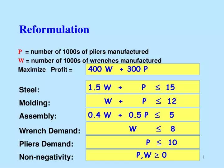
Reformulation. P = number of 1000s of pliers manufactured W = number of 1000s of wrenches manufactured Maximize Profit =. 400 W + 300 P. 1.5 W + P £ 15. Steel:. W + P £ 12. Molding:. 0.4 W + 0.5 P £ 5. Assembly:. W £ 8. Wrench Demand:.

E N D
Reformulation P = number of 1000s of pliers manufactured W= number of 1000s of wrenches manufactured Maximize Profit = 400 W + 300 P 1.5 W + P £ 15 Steel: W + P £ 12 Molding: 0.4 W + 0.5 P £ 5 Assembly: W £ 8 Wrench Demand: P £ 10 Pliers Demand: P,W 0 Non-negativity:
Binding constraints Optimal Solution Structure P Maximize z = 400W + 300P 1.5 W + P £ 15 steel .4W + .5P 5 assembly plus other constraints 14 12 10 8 A constraint is said to be bindingif it holds with equality at the optimum solution. Other constraints arenon-binding 6 4 2 W 2 4 6 8 10 12 14 2
Maximize z = 400W + 300P 1.5W + P = 15 .4W + .5P = 5 How do we find an optimal solution? Optimal solutions occur at corner points. In two dimensions, this is the intersection of 2 lines. P 14 12 10 8 Solution: .7W = 5, W = 50/7 P = 15 - 75/7 = 30/7 z = 29,000/7 = 4,142 6/7 6 4 2 W 2 4 6 8 10 12 14 3
Finding an optimal solution in two dimensions: Summary • The optimal solution (if one exists) occurs at a “corner point” of the feasible region. • In two dimensions with all inequality constraints, a corner point is a solution at which two (or more) constraints are binding. • There is always an optimal solution that is a corner point solution (if a feasible solution exists). • More than one solution may be optimal in some situations
Preview of the Simplex Algorithm • In ndimensions, one cannot evaluate the solution value of every extreme point efficiently. (There are too many.) • The simplex method finds the best solution by a neighborhood search technique. • Two feasible corner points (in 2 dimensions) are said to be “adjacent” (or neighbors) if they have one binding constraint in common.
2 4 6 8 10 12 14 Preview of the Simplex Method P Maximizez = 400W + 300P Start at any feasible extreme point. Move to an adjacent extreme point with better objective value. Continue until no adjacent extreme point has a better objective value. W 2 4 6 8 10 12 14 6
Preview of Sensitivity Analysis P Suppose slightly more steel is available? 1.5W + P 15 +D 14 12 10 What is the impact on the optimal solution value? 8 6 4 2 W 2 4 6 8 10 12 14 7
Shifting a Constraint P Steel is increased to 15 +D. What happens to the optimal solution? What happens to the optimal solution value? 5 4 3 W 6 7 8 8
Shifting a Constraint P Steel is increased to15 +D. What happens to the optimal solution? What happens to the optimal solution value? 5 4 3 W 6 7 8 9
Finding the New Optimum Solution Maximize z = 400W + 300P Binding Constraints: 1.5W + P = 15 +D .4W + .5P = 5 W = 50/7 +(10/7)D P= 30/7 -8/7D z = 29,000/7 +(1,600/7)D Solution: Conclusion: If the amount of steel increases by D units (for sufficiently smallD) then the optimal objective value increases by(1,600/7)D. Theshadow priceof a constraint is the unit increase in the optimal objective value per unit increase in the RHS of the constraint. Thus the shadow price of steel is 1,600/7 = 228 4/7.
Some Questions on Shadow Prices • Suppose the amount of steel was decreased byD units. What is the impact on the optimum objective value? • How large can the increase in steel availability be so that the shadow price remains as 228 4/7? • Suppose that steel becomes available at $1200 per ton. Should you purchase the steel? • Suppose that you could purchase 1 ton of steel for $450. Should you purchase the steel? (Assume here that this is the correct market value for steel.)
Bounds on RHS coefficients in Sensitivity Analysis • Recall that the optimum solution is a corner point, which in 2 dimensions is the solution of 2 equations in 2 variables, and the equations are the binding constraints. • Compute the largest changes in the RHS coefficient so that all constraints remain satisfied.
Shifting a Constraint GTC P Steel is increased to 15 + D. What happens to the optimal solution? Recall that W <= 8. 5 4 The structure of the optimum solution changes when D = .6, and W is increased to 8 3 W 6 7 8 13
Changing the RHS coefficient Increase steel from 15 to 15 + D 1.5 W + P £ 15 1.5 W + P = 15 + D Binding Constraint W + P £ 12 0.4 W + 0.5 P £ 5 Binding Constraint 0.4 W + 0.5 P = 5 W £ 8 P £ 10 P,W 0 W = 50/7 +(10/7)D; P= 30/7 –(8/7)D
Changing the RHS coefficient Compute changes in the LHS of remaining constraints 1.5 W + P = 15 + D W + P £ 12 W + P = 80/7 + (2/7)D£ 12 0.4 W + 0.5 P £ 5 0.4 W + 0.5 P = 5 W = 50/7 + (10/7)D£ 8 W £ 8 P = 30/7 – (8/7)D£ 10 P £ 10 P,W 0 50/7 +(10/7)D 0; 30/7 –(8/7)D 0 W = 50/7 +(10/7)D; P= 30/7 –(8/7)D
Changing the RHS coefficient Compute upper and lower bounds on D 1.5 W + P = 15 + D D£ 2 80/7 + (2/7)D£ 12 0.4 W + 0.5 P £ 5 0.4 W + 0.5 P = 5 50/7 + (10/7)D£ 8 D£ 3/5 W £ 8 30/7 – (8/7)D£ 10 D -5 P £ 10 50/7 +(10/7)D 0; P,W 0 D -5 30/7 –(8/7)D 0 D£ 15/4 So, -5 £ D£ 3/5
Summary for changes in RHS coefficients • Determine the binding constraints • Determine the change in the “corner point solution” as a function of D. • Compute the largest and smallest values of D so that the solution stays feasible. • The shadow price is valid so long as the “corner point solution” remains optimal, which is so long as it is feasible. • If there are three binding constraints, then choose two of these to get the two equations to solve, and the technique still works. (But the change in the solution as a function of D depends on which two constraints are chosen.)
Bounds on Cost coefficients in Sensitivity Analysis • Recall that the optimum solution is a corner point, which in 2 dimensions is the solution of 2 equations in 2 variables, and the equations are the binding constraints. • The solution has two neighboring corner point solutions • Compute the largest changes in the cost coefficient so that the current corner point solution has a better objective value than its neighboring corner point solutions.
P 10 8 6 4 2 .4W + .5P = 5 W 2 4 6 8 10 Shifting a Cost Coefficient GTC The objective is: Maximize z = 400W + 300P What happens to the optimal solution if300Pis replaced by(300+d)P How large can d be for your answer to stay correct? 19
P 10 8 6 4 2 W 2 4 6 8 10 Determining Bounds on Cost Coefficients z = 400W + (300+d) P W = 0; P= 10; z = 3000 + 10 d W = 50/7; P= 30/7; z = 29,000/7 + 30 d /7 W = 8; P= 3; z = 4100 + 3 d
P 10 8 6 4 2 W 2 4 6 8 10 z = 29,000/7 + 30 d /7 4100 + 3 d d -100/3 Determining Bounds on Cost Coefficients W = 0; P= 10; z = 3000 + 10 d z = 29,000/7 + 30 d /7 3000 + 10 d d £ 200 W = 50/7; P= 30/7; z = 29,000/7 + 30 d /7 W = 8; P= 3; z = 4100 + 3 d
Summary: 2D Geometry helps guide the intuition • The Geometry of the Feasible Region • Graphing the constraints • Finding an optimal solution • Graphical method • Searching all the extreme points • Simplex Method • Sensitivity Analysis • Changing the RHS • Changing the Cost Coefficients