Download
1 / 8
80 likes | 225 Views
The Smith Chart is a superposition of two coordinate systems:. z = 0.3 – j1. r = 0.3. x = -1. A constant chart which is linear in distance. A constant r-x chart which is not linear in distance. | |. . 0.5.

E N D
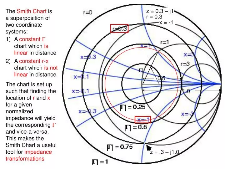
The Smith Chart is a superposition of two coordinate systems: z = 0.3 – j1 r = 0.3 x = -1 • A constant chart which is linear in distance • A constant r-x chart which is not linear in distance || 0.5 The chart is set up such that finding the location of r and x for a given normalized impedance will yield the corresponding and vice-a-versa. This makes the Smith Chart a useful tool for impedance transformations 1.0 z = .3 – j1.0
The standing wave ratio is read off of the chart by noting the r value where a constant circle intersects the r axis • SWR = Zmax/Z0 • = zmax • = rmax • SWR = Z0/Zmin • = 1/zmin • = 1/rmin 1/SWR SWR
POC PSC b values g values -b values
WTG = .14 To convert from zL to yl we can either: • Rotate around constant by /4 (180°) /4 zL • Draw a line from zL through origin until it intersects constant yL WTG = .39
We can transform z into y by rotating z half way around a constant circle Given Z = 95+j20 on a 50 line, find Y • Find z • z = 1.9+j0.4 • Draw circle • Draw line through • origin • Find intersection • with circle • Read off y • y = 0.5-j0.1 • Renormalize y • Y = y/Z0 • = 10-j2 mS • Ycalc = 10.1-j2.12 mS
A 50- T-L is terminated in an impedance of ZL = 35 - j47.5. Find the position and length of the short-circuited stub to match it. WTG = .109 WTG = .168 yL • Normalize ZL • zL = 0.7 – j0.95 yA • Find zL on S.C. • Draw circle • Convert to yL • Find g=1 circle • Find intersection of circle and g=1 circle (yA) • Find distance traveled (WTG) to get to this admittance zL • This is dSTUB • dSTUB = (.168-.109) • dSTUB = .059
A 50- T-L is terminated in an impedance of ZL = 35 - j47.5. Find the position and length of the short-circuited stub to match it. bA = 1.2 • Find bA • Locate PSC yA • Set bSTUB =bA and find ySTUB = -jbSTUB WTG = 0.25 • Find distance traveled (WTG) to get from PSCto bSTUB PSC • This is LSTUB • LSTUB = (0.361-0.25) • LSTUB = .111 Our solution is to place a short-circuited stub of length .111 a distance of .059 from the load. ySTUB = -1.2 WTG = 0.361
There is a second solution where the circle and g=1 circle intersect. This is also a solution to the problem, but requires a longer dSTUB and LSTUB so is less desireable, unless practical constraints require it. WTG = .109 yL yA1 dSTUB = (.332-.109) dSTUB = .223 LSTUB = (.25+.139) LSTUB = .389 yA2 zL WTG = .332