Download
1 / 70
700 likes | 909 Views
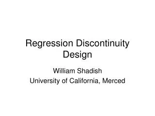
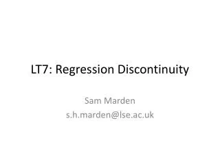
Regression Discontinuity Design. Pr(X i =1 | z). 1. Fuzzy Design. Sharp Design. 0. Z 0. Z. E[Y|Z=z]. E[Y 1 |Z=z]. E[Y 0 |Z=z]. Z 0. Y. y(z 0 )+ α. y(z 0 ). z. z 0 -2h 1. z 0 -h 1. z 0 +h 1. z 0 +2h 1. z 0. Motivating example.

E N D
Pr(Xi=1 | z) 1 Fuzzy Design Sharp Design 0 Z0 Z
E[Y|Z=z] E[Y1|Z=z] E[Y0|Z=z] Z0
Y y(z0)+α y(z0) z z0-2h1 z0-h1 z0+h1 z0+2h1 z0
Motivating example • Many districts have summer school to help kids improve outcomes between grades • Enrichment, or • Assist those lagging • Research question: does summer school improve outcomes • Variables: • x=1 is summer school after grade g • y = test score in grade g+1
LUSDINE • To be promoted to the next grade, students need to demonstrate proficiency in math and reading • Determined by test scores • If the test scores are too low – mandatory summer school • After summer school, re-take tests at the end of summer, if pass, then promoted
Situation • Let Z be test score – Z is scaled such that • Z≥0 not enrolled in summer school • Z<0 enrolled in summer school • Consider two kids • #1: Z=ε • #2: Z=-ε • Where ε is small
Intuitive understanding • Participants in SS are very different • However, at the margin, those just at Z=0 are virtually identical • One with z=-ε is assigned to summer school, but z= ε is not • Therefore, we should see two things
There should be a noticeable jump in SS enrollment at z=0. • If SS has an impact on test scores, we should see a jump in test scores at z=0 as well.
Variable Definitions • yi = outcome of interest • xi =1 if NOT in summer school, =1 if in • Di = I(zi≥0) -- I is indicator function that equals 1 when true, =0 otherwise • zi = running variable that determines eligibility for summer school. z is re-scaled so that zi=0 for the lowest value where Di=1 • wi are other covariates
Key assumption of RDD models • People right above and below Z0 are functionally identical • Random variation puts someone above Z0 and someone below • However, this small different generates big differences in treatment (x) • Therefore any difference in Y right at Z0 is due to x
Limitation • Treatment is identified for people at the zi=0 • Therefore, model identifies the effect for people at that point • Does not say whether outcomes change when the critical value is moved
RD Estimates Fixed Effects Results
* eligible for Medicare after quarter 259; gen age65=age_qtr>259; * scale the age in quarters index so that it equals 0; * in the month you become eligible for Medicare; gen index=age_qtr-260; gen index2=index*index; gen index3=index*index*index; gen index4=index2*index2; gen index_age65=index*age65; gen index2_age65=index2*age65; gen index3_age65=index3*age65; gen index4_age65=index4*age65; gen index_1minusage65=index*(1-age65); gen index2_1minusage65=index2*(1-age65); gen index3_1minusage65=index3*(1-age65); gen index4_1minusage65=index4*(1-age65);
* 1st stage results. Impact of Medicare on insurance coverage; * basic results in the paper. cubic in age interacted with age65; * method 1; reg insured male white black hispanic _I* index index2 index3 index_age65 index2_age65 index3_age65 age65, cluster(index); * 1st stage results. Impact of Medicare on insurance coverage; * basic results in the paper. quadratic in age interacted with; * age65 and 1-age65; * method 2; reg insured male white black hispanic _I* index_1minus index2_1minus index3_1minus index_age65 index2_age65 index3_age65 age65, cluster(index);
Method 1 Linear regression Number of obs = 46950 F( 21, 79) = 182.44 Prob > F = 0.0000 R-squared = 0.0954 Root MSE = .25993 (Std. Err. adjusted for 80 clusters in index) ------------------------------------------------------------------------------ | Robust insured | Coef. Std. Err. t P>|t| [95% Conf. Interval] -------------+---------------------------------------------------------------- male | .0077901 .0026721 2.92 0.005 .0024714 .0131087 white | .0398671 .0074129 5.38 0.000 .0251121 .0546221 delete some results index | .0006851 .0017412 0.39 0.695 -.0027808 .0041509 index2 | 1.60e-06 .0001067 0.02 0.988 -.0002107 .0002139 index3 | -1.42e-07 1.79e-06 -0.08 0.937 -3.71e-06 3.43e-06 index_age65 | .0036536 .0023731 1.54 0.128 -.0010698 .0083771 index2_age65 | -.0002017 .0001372 -1.47 0.145 -.0004748 .0000714 index3_age65 | 3.10e-06 2.24e-06 1.38 0.171 -1.36e-06 7.57e-06 age65 | .0840021 .0105949 7.93 0.000 .0629134 .1050907 _cons | .6814804 .0167107 40.78 0.000 .6482186 .7147422 ------------------------------------------------------------------------------
Method 2 Linear regression Number of obs = 46950 F( 21, 79) = 182.44 Prob > F = 0.0000 R-squared = 0.0954 Root MSE = .25993 (Std. Err. adjusted for 80 clusters in index) ------------------------------------------------------------------------------ | Robust insured | Coef. Std. Err. t P>|t| [95% Conf. Interval] -------------+---------------------------------------------------------------- male | .0077901 .0026721 2.92 0.005 .0024714 .0131087 white | .0398671 .0074129 5.38 0.000 .0251121 .0546221 delete some results index_1mi~65 | .0006851 .0017412 0.39 0.695 -.0027808 .0041509 index2_1m~65 | 1.60e-06 .0001067 0.02 0.988 -.0002107 .0002139 index3_1m~65 | -1.42e-07 1.79e-06 -0.08 0.937 -3.71e-06 3.43e-06 index_age65 | .0043387 .0016075 2.70 0.009 .0011389 .0075384 index2_age65 | -.0002001 .0000865 -2.31 0.023 -.0003723 -.0000279 index3_age65 | 2.96e-06 1.35e-06 2.20 0.031 2.79e-07 5.65e-06 age65 | .0840021 .0105949 7.93 0.000 .0629134 .1050907 _cons | .6814804 .0167107 40.78 0.000 .6482186 .7147422 ------------------------------------------------------------------------------
Oreopoulos, AER • Enormous interest in the rate of return to education • Problem: • OLS subject to OVB • 2SLS are defined for small population (LATE) • Comp. schooling, distance to college, etc. • Maybe not representative of group in policy simulations) • Solution: LATE for large group
School reform in GB (1944) • Raised age of comp. schooling from 14 to 15 • Effective 1947 (England, Scotland, Wales) • Raised education levels immediately • Concerted national effort to increase supplies (teachers, buildings, furniture) • Northern Ireland had similar law, 1957
1-39 students, one class • 40-79 students, 2 classes • 80 to 119 students, 3 classes • Addition of one student can generate large changes in average class size