Download
1 / 75
750 likes | 982 Views
V9: Reliability of Protein Interaction Networks. One would like to integrate evidence from many different sources to increase the predictivity of true and false protein-protein predictions.

E N D
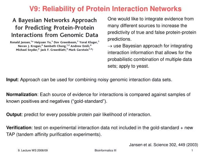
V9: Reliability of Protein Interaction Networks One would like to integrate evidence from many different sources to increase the predictivity of true and false protein-protein predictions. use Bayesian approach for integrating interaction information that allows for the probabilistic combination of multiple data sets; apply to yeast. Input: Approach can be used for combining noisy genomic interaction data sets. Normalization: Each source of evidence for interactions is compared against samples of known positives and negatives (“gold-standard”). Output: predict for every possible protein pair likelihood of interaction. Verification: test on experimental interaction data not included in the gold-standard + new TAP (tandem affinity purification experiments). Jansen et al. Science 302, 449 (2003) Bioinformatics III
Integration of various information sources 3 different types of data used: (i) Interaction data from high-throughput experiments. These comprise large-scale two-hybrid screens (Y2H) and in vivo pull-down experiments. (ii) Other genomic features: expression data, biological function of proteins (from Gene Ontology biological process and the MIPS functional catalog), and data about whether proteins are essential. (iii) Gold-standards of known interactions and noninteracting protein pairs. Jansen et al. Science 302, 449 (2003) Bioinformatics III
Combination of data sets into probabilistic interactomes The 4 interaction data sets from HT experiments were combined into 1 PIE. The PIE represents a transformation of the individual binary-valued interaction sets into a data set where every protein pair is weighed according to the likelihood that it exists in a complex. (B) Combination of data sets into probabilistic interactomes. A „naïve” Bayesian network is used to model the PIP data. These information sets hardly overlap. Because the 4 experimental interaction data sets contain correlated evidence, a fully connected Bayesian network is used. Jansen et al. Science 302, 449 (2003) Bioinformatics III
Bayesian Networks Bayesian networks are probabilistic models that graphically encode probabilistic dependencies between random variables. Y A directed arc between variables Y and E1 denotes conditional dependency of E1 on Y, as determined by the direction of the arc. E1 E3 E2 Bayesian networks also include a quantitative measure of dependency. For each variable and its parents this measure is defined using a conditional probability function or a table. Here, one such measure is the probability Pr(E1|Y). Bioinformatics III
Bayesian Networks Together, the graphical structure and the conditional probability functions/tables completely specify a Bayesian network probabilistic model. Y This model, in turn, specifies a particular factorization of the joint probability distribution function over the variables in the networks. E1 E3 E2 Here, Pr(Y,E1,E2,E3) = Pr(E1|Y) Pr(E2|Y) Pr(E3|Y) Pr(Y) Bioinformatics III
Gold-Standard should be (i) independent from the data sources serving as evidence (ii) sufficiently large for reliable statistics (iii) free of systematic bias (e.g. towards certain types of interactions). Positives: use MIPS (Munich Information Center for Protein Sequences, HW Mewes) complexes catalog: hand-curated list of complexes (8250 protein pairs that are within the same complex) from biomedical literature. Negatives: - harder to define - essential for successful training Assume that proteins in different compartments do not interact. Synthesize “negatives” from lists of proteins in separate subcellular compartments. Jansen et al. Science 302, 449 (2003) Bioinformatics III
Measure of reliability: likelihood ratio Consider a genomic feature f expressed in binary terms (i.e. „absent“ or „present“). Likelihood ratio L(f) is defined as: L(f) = 1 means that the feature has no predictability: the same number of positives and negatives have feature f. The larger L(f) the better its predictability. Jansen et al. Science 302, 449 (2003) Bioinformatics III
Combination of features For two features f1and f2 with uncorrelated evidence, the likelihood ratio of the combined evidence is simply the product: L(f1,f2) = L(f1) L(f2) For correlated evidence L(f1,f2) cannot be factorized in this way. Bayesian networks are a formal representation of such relationships between features. The combined likelihood ratio is proportional to the estimated odds that two proteins are in the same complex, given multiple sources of information. Jansen et al. Science 302, 449 (2003) Bioinformatics III
Prior and posterior odds „positive“ : a pair of proteins that are in the same complex. Given the number of positives among the total number of protein pairs, the „prior“ odds of finding a positive are: „posterior“ odds: odds of finding a positive after considering N datasets with values f1 ... fN : The terms „prior“ and „posterior“ refer to the situation before and after knowing the information in the N datasets. Jansen et al. Science 302, 449 (2003) Bioinformatics III
Static naive Bayesian Networks In the case of protein-protein interaction data, the posterior odds describe the odds of having a protein-protein interaction given that we have the information from the N experiments, whereas the prior odds are related to the chance of randomly finding a protein-protein interaction when no experimental data is known. If Opost> 1, the chances of having an interaction are higher than having no interaction. Jansen et al. Science 302, 449 (2003) Bioinformatics III
Static naive Bayesian Networks The likelihood ratio L defined as relates prior and posterior odds according to Bayes‘ rule: In the special case that the N features are conditionally independent (i.e. they provide uncorrelated evidence) the Bayesian network is a so-called „naïve” network, and L can be simplified to: Jansen et al. Science 302, 449 (2003) Bioinformatics III
Computation of prior and posterior odds L can be computed from contingency tables relating positive and negative examples with the N features (by binning the feature values f1 ... fNinto discrete intervals). Determining the prior odds Oprioris somewhat arbitrary. It requires an assumption about the number of positives. Here, 30,000 is taken a conservative lower bound for the number of positives (i.e. pairs of proteins that are in the same complex). Considering that there are ca. 18 million = 0.5 * N (N – 1) possible protein pairs in total (with N = 6000 for yeast), Opost > 1 can be achieved with L > 600. Jansen et al. Science 302, 449 (2003) Bioinformatics III
Essentiality (PIP) Consider whether proteins are essential or non-essential = does a deletion mutant where this protein is knocked out from the genome have the same phenotype? It should be more likely that both of 2 proteins in a complex are essential or non-essential, but not a mixture of these two attributes. Deletion mutants of either one protein should impair the function of the same complex. Jansen et al. Science 302, 449 (2003) Bioinformatics III
Parameters of the naïve Bayesian Networks (PIP) Column 1 describes the genomic feature. In the „essentiality data“ protein pairs can take on 3 discrete values (EE: both essential; NN: both non-essential; NE: one essential and one not). Column 2 gives the number of protein pairs with a particular feature (i.e. „EE“) drawn from the whole yeast interactome (~18M pairs). Columns „pos“ and „neg“ give the overlap of these pairs with the 8,250 gold-standard positives and the 2,708,746 gold-standard negatives. Columns „sum(pos)“ and „sum(neg)“ show how many gold-standard positives (negatives) are among the protein pairs with likelihood ratio L, computed by summing up the values in the „pos“ (or „neg“) column. P(feature value|pos) and P(feature value|neg) give the conditional probabilities of the feature values – and L, the ratio of these two conditional probabilities. Jansen et al. Science 302, 449 (2003) Bioinformatics III
mRNA expression data Proteins in the same complex tend to have correlated expression profiles. Although large differences can exist between the mRNA and protein abundance, protein abundance can be indirectly and quite crudely measured by the presence or absence of the corresponding mRNA transcript. Experimental data source: - time course of expression fluctuations during the yeast cell cycle - Rosetta compendium: expression profiles of 300 deletion mutants and cells under chemical treatments. Problem: both data sets are strongly correlated. Compute first principal component of the vector of the 2 correlations. Use this as independent source of evidence for the P-P interaction prediction. The first principal component is a stronger predictor of P-P interactions that either of the 2 expression correlation datasets by themselves. Jansen et al. Science 302, 449 (2003) Bioinformatics III
mRNA expression data The values for mRNA expression correlation (first principal component) range on a continuous scale from -1.0 to +1.0 (fully anticorrelated to fully correlated). This range was binned into 19 intervals. Jansen et al. Science 302, 449 (2003) Bioinformatics III
PIP – Functional similarity Quantify functional similarity between two proteins: - consider which set of functional classes two proteins share, given either the MIPS or Gene Ontology (GO) classification system. - Then count how many of the ~18 million protein pairs in yeast share the exact same functional classes as well (yielding integer counts between 1 and ~ 18 million). It was binned into 5 intervals. - In general, the smaller this count, the more similar and specific is the functional description of the two proteins. Jansen et al. Science 302, 449 (2003) Bioinformatics III
PIP – Functional similarity Observation: low counts correlate with a higher chance of two proteins being in the same complex. But signal (L) is quite weak. Jansen et al. Science 302, 449 (2003) Bioinformatics III
Calculation of the fully connected Bayesian network (PIE) The 3 binary experimental interaction datasets can be combined in at most 24 = 16 different ways (subsets). For each of these 16 subsets, one can compute a likelihood ratio from the overlap with the gold-standard positives („pos“) and negatives („neg“). Jansen et al. Science 302, 449 (2003) Bioinformatics III
Distribution of likelihood ratios Number of protein pairs in the individual datasets and the probabilistic interactomes as a function of the likelihood ratio. There are many more protein pairs with high likelihood ratios in the probabilistic interactomes (PIE) than in the individual datasets G,H,U,I. Protein pairs with high likelihood ratios provide leads for further experimental investigation of proteins that potentially form complexes. Jansen et al. Science 302, 449 (2003) Bioinformatics III
PIP vs. the information sources Ratio of true to false positives (TP/FP) increases monotonically with Lcut. L is an appropriate measure of the odds of a real interaction. The ratio is computed as: Protein pairs with Lcut > 600 have a > 50% chance of being in the same complex. Jansen et al. Science 302, 449 (2003) Bioinformatics III
PIE vs. the information sources 9897 interactions are predicted from PIP and 163 from PIE. In contrast, likelihood ratios derived from single genomic factors (e.g. mRNA coexpression) or from individual interaction experiments (e.g. the Ho data set) did no exceed the cutoff when used alone. This demonstrates that information sources that, taken alone, are only weak predictors of interactions can yield reliable predictions when combined. Jansen et al. Science 302, 449 (2003) Bioinformatics III
parts of PIP graph Test whether the thresholded PIP was biased toward certain complexes, compare distribution of predictions among gold-standard positives. (A ) The complete set of gold-standard positives and their overlap with the PIP. The PIP (green) covers 27% of the gold-standard positives (yellow). The predicted complexes are roughly equally apportitioned among the different complexes no bias. Jansen et al. Science 302, 449 (2003) Bioinformatics III
parts of PIP graph Graph of the largest complexes in PIP, i.e. only those proteins having 20 links. (Left) overlapping gold-standard positives are shown in green, PIE links in blue, and overlaps with both PIE and gold-standard positives in black. (Right) Overlapping gold-standard negatives are shown in red. Regions with many red links indicate potential false-positive predictions. Jansen et al. Science 302, 449 (2003) Bioinformatics III
experimental verification conduct TAP-tagging experiments (Cellzome) for 98 proteins. These produced 424 experimental interactions overlapping with the PIP threshold at Lcut = 300. Of these, 185 overlapped with gold-standard positives and 16 with negatives. Jansen et al. Science 302, 449 (2003) Bioinformatics III
Concentrate on large complexes Sofar all interactions were treated as independent. However, the joint distribution of interactions in the PIs can help identify large complexes: an ideal complex should be a fully connected „clique“ in an interaction graph. In practice, this rarely happens because of incorrect or missing links. Yet large complexes tend to have many interconnections between them, whereas false-positive links to outside proteins tend to occur randomly, without a coherent pattern. Jansen et al. Science 302, 449 (2003) Bioinformatics III
Improve ratio TP / FP TP/FP for subsets of the thresholded PIP that only include proteins with a minimum number of links. Requiring a minimum number of links isolates large complexes in the thresholded PIP graph (Fig. 3B). Observation: Increasing the minimum number of links raises TP/FP by preserving the interactions among proteins in large complexes, while filtering out false-positive interactions with heterogeneous groups of proteins outside the complexes. Jansen et al. Science 302, 449 (2003) Bioinformatics III
Summary Bayesian approach allows reliable predictions of protein-protein interactions by combining weakly predictive genomic features. The de novo prediction of complexes replicated interactions found in the gold-standard positives and PIE. Also, several predictions were confirmed by new TAP experiments. The accuracy of the PIP was comparable to that of the PIE while simultaneously achieving greater coverage. In a similar manner, the approach could have been extended to a number of other features related to interactions (e.g. phylogenetic co-occurrence, gene fusions, gene neighborhood). As a word of caution: Bayesian approaches don‘t work everywhere. Jansen et al. Science 302, 449 (2003) Bioinformatics III
Dynamic Simulation of Protein Complex Formation • - Most cellular functions are conducted or regulated by protein complexes of varying size • organization into complexes may contribute substantially to an organism‘s complexity. • E.g. 6000 different proteins (yeast) may form 18 106 different pairs of interacting proteins, but already 1011 different complexes of size 3. • mechanism how evolution could significantly increase the regulatory and metabolic complexity of organisms without substantially increasing the genome size. • - Only a very small subset of the many possible complexes is actually realized. Beyer, Wilhelm, Bioinformatics Bioinformatics III
Experimental reference data 229 biologically meaningful ‚TAP complexes‘ from yeast with sizes ranging from 2 to 88 different proteins per complex. „Cumulative“ means that there are 229 complexes of size 2 that may also be parts of larger complexes. size-frequency of complexes has common characteristics: # of complexes of a given size versus complex size is exponentially decreasing Does the shape of this distribution reflect the nature of the underlying cellular dynamics which is creating the protein complexes? Test by simulation model Bioinformatics III
Dynamic Complex Formation Model 3 variants of the protein complex association-dissociation model (PAD-model) are tested with the following features: (i) In all 3 versions the composition of the proteome does not change with time. Degradation of proteins is always balanced by an equal production of the same kind of proteins. (ii) The cell consists of either one (PAD A & B) or several (PAD C) compartments in which proteins and protein complexes can freely interact with each other. Thus, all proteins can potentially bind to all other proteins in their compartment (risky assumption!). (iii) Association and dissociation rate constants are the same for all proteins. In PAD-models A and C association and dissociation are independent of complex size and complex structure. Bioinformatics III
Dynamic Complex Formation Model (iv) At each time step a set of complexes is randomly selected to undergo association and dissociation. Association is simulated as the creation of new complexes by the binding of two smaller complexes. Dissociation is simulated as the reverse process, i.e. it is the decay of a complex into two smaller complexes. The number of associations and dissociations per time step are ka· NC2and kd · NCrespectively, NC: total number of complexes in the cell ka[1/(#complexes · time)] : association rate constant kd[1/time] : dissociation rate constant. kaand kdcorrespond to the biochemical rates of a reversible reaction. Bioinformatics III
Protein Association/Dissociation Models PAD A: the most simple model where all proteins can interact with each other (no partitioning) and it assumes that association and dissociation are independent of complex size. PAD B : is equivalent to PAD A, but larger complexes are assumed more likely to bind (preferential attachment). Here, the binding probability is assumed as proportional to i·j, where i and j are the sizes of two potentially interacting complexes. PAD C : extends PAD A by assuming that proteins can interact only withingroups of proteins (with partitioning). The sizes of these protein groups are based on the sizes of first level functional modules according to the yeast data base. PAD C assumes 16 modules each containing between 100 and 1000 different ORFs. the protein groups do not represent physical compartments, but rather resemble functional modules of interacting proteins. Bioinformatics III
Mathematical Description - explicit simulation of an entire cell (50 million protein molecules were simulated) is too time consuming for many applications of the model. - therefore use a simplified mathematical description of the PAD model to quickly assess different scenarios and parameter combinations. The change of the number of complexes of size i, xi, during one time step t can be described as (1) Giaand Gid : gains due to association and dissociation L i aand Lid : losses due to association and dissociation Bioinformatics III
Mathematical Description Given a total number of NCcomplexes, the total number of associations and dissociations per time step are ka · NC2and k d · NC, respectively. We assume throughout that we can calculate the mean number of associating or dissociating complexes of size i per time step as 2 · ka · xi· NCand kd · xi. The probability that complexes of size j and i-j get selected for one association is deduce the number of complexes of size i that get created during each time step via association of smaller complexes simply by summing over all complex sizes that potentially create a complex of size i: Bioinformatics III
Mathematical Description When j is equal to i/2 (which is possible only for even i’s) both interaction partners have the same size. The size of the pool xi-j is therefore reduced by 1 after the first interaction partner has been selected, which yields a small reduction of the probability of selecting a second complex from that pool. Account for this effect with the correction i, which only applies to even i’s: This correction is usually very small. The loss of complexes of size i due to association is simply proportional to the probability of selecting them for association, i.e. Bioinformatics III
Mathematical Description Complexes of size i get created by dissociation of larger complexes. A complex of size j has possible ways of dissociation and the number of possible fragments of size i is The probability that a dissociating complex of size j > i creates a fragment of size i is hence The number of new complexes follows by summing over all possible parent sizes The respective loss term becomes Bioinformatics III
Number of complexes formed The figure shows a comparison of a numerical solution of equation (1) with a stochastic simulation of the association-dissociation process. Bioinformatics III
Steady-state After a transient period a steady-state is reached. We are mainly interested in this steady-state distribution of frequencies xi. find a set of xisolving xi/t = 0. The solution of this non-linear equation system is obtained by numerically minimizing all xi /t. By dividing equation (1) by kdit can be seen that the steady-state distribution is independent of the absolute values of kaand kd, but it only depends on the ratio of the two parameters Rad= ka/ kd. Hence, only two parameters affect the xiat steady-state: - the total number of proteins NP(which indirectly determines NC) and - the ratio of the two rate constants Rad. Bioinformatics III
Association in model C For PAD-model B the dissociation terms remain unchanged, wheras the association terms have to be modified. In case of PAD C we calculated weighted averages of results obtained with PAD A. Assume that association is proportional to the product of the sizes of the participating complexes. This assumption changes equation (2) to: where n is the maximum complex size and Bioinformatics III
Computation of a Dissociation Constant KD Mathematically our model describes a reversible (bio-)chemical reaction. calculate an equilibrium dissociation constant KD, which quantifies the fraction of free subcomplexes A and B compared to the bound complex AB. This equilibrium is complex size dependent, because a large complex AB is less likely to randomly dissociate exactly into the two specific subunits A and B than a small complex. (A and B can be ensembles of several proteins.) We get for any given complex of size i the following KD: KD(i) = [A][B] / [AB] = (Rad·Ni· V) – 1 (4) where Niis the number of possible fragments of a complex of size i and V is the cell volume. Cell-wide averages of KD-values are estimated by computing a weighted average with NCbeing the total number of complexes and xibeing the number of complexes of size i. Bioinformatics III
Results - dynamically simulate the association and dissociation of 6200 different protein types yielding a set of about 50 million protein molecules. - analyze the resulting steady-state size distribution of protein complexes. This steady-state is thought to reflect the growth conditions under which the yeast cells were held when TAP-measuring the protein complexes. - calculate a protein complex size distribution from the exp. data to which we can compare the simulation results (Figure 1). Bioinformatics III
Results TAP measurements do not provide concentrations of the measured complexes, they only demonstrate the presence of a certain protein complex in yeast cells. Also the number of proteins of a certain type inside such a complex could not be measured the complex size from Figure 1 does not represent real complex sizes (i.e. total number of proteins in the complex), but it refers to the number of different proteins in a complex. The measured data reflect the characteristics of only 229 different protein complexes of size 2, which is just a small subset of the ‘complexosome’. These peculiarities have to be taken into account when comparing simulation results to the observed complex size distribution. Here, the ‘measurable complex size’ is taken as the number of distinct proteins in a protein complex (Figure 2). When comparing our simulation results to the measurements, we always select a random-subset of 229 different complexes from the simulated pool of complexes. This results in a complex size distribution comparable to the measured distribution from Figure 1 (‘bait distribution’). Bioinformatics III
Effect of preferential attachment Both simulations were performed with the best fit parameters for PAD A. In case of preferential attachment the best regression result (solid line) is obtained with a power-law, while the simulation without preferential attachment is best fitted assuming an exponentially decreasing curve. The original, measurable and bait distributions are always close to exponential in case of PAD A and power-law like in case of PAD B, independent of the parameters chosen. Cumulative number of distinct protein complexes versus their size, resulting from simulations without (diamonds) and with (squares) preferential attachment to larger complexes. PAD B model gives power-law distribution not in agreement with experimental observation. Bioinformatics III
Conclusions A very simple, dynamic model can reproduce the observed complex size distribution. Given the small number of input parameters the very good fit of the observed data is astonishing (and may be fortuitous). Preferential attachment does not take place in yeast cells under the investigated conditions. This is biologically plausible: Specific and strong binding can be just as important for small protein complexes as for large complexes. the dissociation should on average be independent of the complex size. Interpreting the simulated association and dissociation in terms of KD-values suggests that larger complexes bind more strongly than smaller complexes. However, the size dependence of KDis compensated by the higher number of possible dissociations in larger complexes. Here, we assumed that all possible dissociations happen with the same probability. In reality large complexes may break into specific subcomplexes, which subsequently can be re-used for a different purpose. Improved versions of the model should account for specificity of association and for specific dissociation. Bioinformatics III
Conclusions Conclusion 2 the number of complexes that were missed during the TAP measurements is potentially large. Simulations give an upper limit of the number of different complexes in cells. At a first glance, the number of different complexes in PAD A (> 3.5 mill.) and PAD C (~ 2 mill.) may appear to be far too large. Even PAD C may overestimate the true number of different complexes, because association within the groups is unrestricted. However, the PAD-models do not only simulate functional, mature complexes, but they also consider all intermediate steps. Each of these steps is counted as a different protein complex. The large difference between the number of measured complexes and the (potential) number of existing complexes may partly explain the very small overlap that has been observed between different large scale measurements of protein complexes. A correct interpretation of the kinetic parameters is important: - kaand kdcannot be compared to real numbers, because the model does not define a length of the time steps for interpreting kaand kdas actual rate constants. - the association-to-dissociation ratio Rad is not identical to a physical KD-value obtained by in vitro measurements of protein binding in water solutions. Bioinformatics III
Discussion Factors complicating this simple interpretation: (i) In vivo diffusion rates are below those in water (e.g. 5 – 20-fold) due to the high concentration of proteins and other large molecules in the cytosol. (ii) Most proteins either are synthesized where they are needed or they get transported directly to the site where the complex gets compiled. transport to the site of action is on average faster than random diffusion. (iii) Protein concentrations are often above the cell average due to the compartmentalization of the cell. All these processes (protein production, transport, and degradation) are not explicitly described in the PAD-model, but they are lumped in the assumptions. The Radmust therefore be interpreted as an operationally defined property. It characterizes the overall, cell averaged complex assembly process, which includes all steps necessary to synthesize a protein complex. Bioinformatics III
Discussion However, even the model-derived KD-s allow for some conclusions regarding complex formation. We calculated weighted averages (KD) of the size-dependent KD-values by using the steady-state complex size distribution of the best fit. This yields average KD -s of 4.7 nM and 0.18 nM for the best fits of PAD A and PAD C, respectively. First, the fact that the KDfor PAD C is below that of PAD A underlines the notion that more specific binding is reflected by smaller KDvalues. Second, typical in vitro KD–values are > 1 nM. Thus the average KDof PAD C is quite low. The model confirms that protein complex formation in vivo gets accelerated due to directed protein transport and due to the compartmentalization of eukaryotes. Bioinformatics III
Discussion The simulated complex size distribution is almost independent of the assumed protein abundance distribution. PPis a valuable summarizing property that can be used to characterize proteomes of different species. A decreasing PPincreases the number of different large complexes (the slope in Table 1 gets more shallow), because it is less likely that a large complex contains the same protein twice. Thus, PPis a measure of complexity that not only relates to the diversity of the proteome but also to the composition of protein complexes. Probably the most severe simplification in our model is the assumption that all proteins can potentially interact with each other. PAD-model C is a first step towards more biological realism. By restricting the number of potential interaction partners it more closely maps functional modules and cell compartments, which both restrict the interaction among proteins. Bioinformatics III
Further improvements The partitioning in PAD C means that proteins within one group exhibit very strong binding, whereas binding between protein groups is set to zero. This again is a simplification, since cross-talk between different modules or compartments is possible. Future extensions of the model could incorporate more and more detailed information about the binding specificity of proteins. Assuming even more specific binding will further reduce the number of different complexes, whereas the frequency of the complexes will increase. High binding specificity potentially lowers the complex sizes, so Radhas to be increased in order to fit the experimentally observed protein complex size distribution. On the other hand, cross talk gives rise to larger complexes. Taking both counteracting refinements into account, it is impossible to generally predict the best-fit Rad, since it depends on the quantitative details. Bioinformatics III