Download

1 / 40
400 likes | 405 Views
Laboratori Nazionali di Frascati, 29 th May 2013. Planck Constraints on the Physics of the Early Universe. Sabino Matarrese Physics & Astronomy Dept. “G. Galilei”, Padova University INFN Sezione di Padova Padova – Italy on behalf of the Planck collaboration.

E N D
Laboratori Nazionali di Frascati, 29th May 2013 Planck Constraints on the Physics of the Early Universe Sabino Matarrese Physics & Astronomy Dept. “G. Galilei”, Padova University INFN Sezione di Padova Padova – Italy on behalf of the Planck collaboration arXiv:1303.5082v1 & arXiv:1303.5084v1
The scientific results that we present today are a product of the Planck Collaboration, including individuals from more than 100 scientific institutes in Europe, the USA and Canada Planck is a project of the European Space Agency, with instruments provided by two scientific Consortia funded by ESA member states (in particular the lead countries: France and Italy) with contributions from NASA (USA), and telescope reflectors provided in a collaboration between ESA and a scientific Consortium led and funded by Denmark.
The Universe thermal history & Inflation INFLATION Inflation is an era of accelerated expansion in the early Universe, driven by the dynamics of a scalar field, the “inflaton”. Small fluctuations in the energy density originated during inflation from quantum vacuum oscillations. These primordial fluctuations originated the CMB temperature anisotripies (and polarization) and provided the seeds of cosmic structure formation. The inflationary era had to occur before baryogenesis took place
Friedmann vs. Newton Robertson-Walker metric scale factor F = ma E = const. M = const.
The Big Bang “crisis” • Horizon problem: does our Universe belong to … a set of measure zero? • Flatness problem: do we need to fine-tune the initial conditions of our Universe? • Cosmic fluctuation problem: how did perturbations come from?
Inflation dynamics I • The vacuum expectation value of the inflaton scalar field behaves like a perfect fluid, but, unlike standard fluids, it can have negative pressure, thus driving a suitable period of accelerated expansion in the early Universe, dubbed “inflation”. If a long enough period of inflation (more than 60 e-folds) occurred it solves the horizon and flatness problem of the Big Bang model and generates the seeds of cosmic structure formation and CMB anisotropies by quantum oscillations of the vacuum state
Inflation dynamics II Different models of inflation derive from different potential and different initial conditions. Old inflation (Guth 1981) assumes thermal initial conditions (which are very difficult to achieve). Chaotic inflation (Linde 1983) is based on the application of the uncertainty principle at Planck energies.
Inflation and the Inflaton Inflation is attained if the energy density of the universe is dominated by the potential energy of a scalar field (the inflaton) The inflaton is slowly rolling along its potential: Slow-roll conditions: the potential V(ϕ) must beflat and
Curvature power-spectrum from inflation • The Planck baseline model assumes purely adiabatic scalar perturbations at very early times, with a (dimensionless) curvature power-spectrum parameterized by with ns and dns/dlnk = const. The baseline model assumes no “running”, i.e. dns/d ln k = 0. The pivot scale k0 = 0.05 Mpc−1. With this choice, ns is not strongly degenerate with the amplitude parameter As.
Tensor-mode power-spectrum • The Planck analysis also considers extended models with a significant amplitude of primordial gravitational waves (tensor modes) with (dimensionless) tensor mode spectrum parameterized as a power-law with • We define r0.05 = At/As, the primordial tensor-to-scalar ratio at k = k0. Our constraints are only weakly sensitive to the tensor spectral index, nt (assumed to be close to zero), and we adopt the theoretically motivated single-field inflation consistency relation nt = - r0.05/8, rather than varying nt independently.
The Planck angular power-spectrum The temperature angular power spectrum (l(l + 1)Cl/2π) of the primary CMB from Planck, showing a precise measurement of 7 acoustic peaks, well fit by a simple 6-parameter ΛCDM model [Planck+WP+highL]. The shaded area around the best-fit curve represents cosmic variance, including sky cut. The error bars on individual points also include cosmic variance. The horizontal axis is logarithmic up to l = 50, and linear beyond. The measured spectrum here is the same as the previous figure, rebinned to show better the low-l region.
Initial (inflationary) conditions • The Planck nominal mission temperature anisotropy measurements, combined with the WMAP large-angle polarization, constrain the scalar spectral index to ns = 0.9603 ± 0.0073, ruling out exact scale invariance at over 5σ. Planck establishes an upper bound on the tensor-to-scalar ratio at r < 0.11 (95% CL). The Planck data shrink the space of allowed standard infla- tionary models, preferring potentials with V” < 0. Exponential potential models, the simplest hybrid inflationary models, and monomial potential models of degree n ≥ 2 do not provide a good fit to the data. Planck does not find statistically significant running of the scalar spectral index, obtaining dns /d ln k = −0.0134 ± 0.0090.
Energy scale of inflation • The Planck constraint on the tensor to scalar ratio r corresponds to an upper bound on the energy scale of inflation at 95 % CL. This in turn is equivalent to an upper bound on the Hubble parameter during inflation
Initial (inflationary) conditions Marginalized joint 68% and 95% CL regions for (r, ns), using Planck+WP+BAO with and without a running spectral index Marginalized joint 68% and 95% CL regions for (d2ns=d ln k2; d ns=d ln k) using Planck+WP+BAO.
Planck constraints in inflation model space • Marginalized joint 68% and 95% CL regions for ns and r0:002 from Planck in combination with other data sets compared to • the theoretical predictions of selected inflationary models Marginalized joint 68% and 95% CL regions for ns and r0.002 from Planck in combination with other data sets compared to the theoretical predictions of selected inflationary models.
Consequences for Inflation models • exponential, simplest hybrid inflation and monomial (V(φ)=φn, n=2,4) do not fit well observations, e.g. n=4 outside the 99.7% CL, n=2 outside 95% CL • Axion monodromy inspired models, as above, with n=1,2/3, lie within 95% CL, and on the boundary of 95% CL respectively. • Hilltop (1-φp/μp) con p=2 in agreement, within 95% CL • natural inflation (1+cos[φ/f]) consistent, for f ≥ 5 MPl • R2 Model (Starobinsky ‘80) consistent with data
Testable predictions of inflation • Cosmological aspects • Critical density Universe • Almost scale-invariant and nearly Gaussian, adiabatic density fluctuations • Almost scale-invariant stochastic background of relic gravitational waves • Particle physics aspects • Nature of the inflaton • Inflation energy scale
Primordial non-Gaussianity: a new route to falsify Inflation ... • Strongly non-Gaussian initial conditions studied in the eighties. • New era with fNL models from inflation (Salopek & Bond 1991; Gangui, Lucchin, Matarrese & Mollerach 1994: fNL~ 10-2; Verde, Wang, Heavens Kamionkowski 2000; Komatsu & Spergel 2001; Acquaviva, Bartolo, Matarrese & Riotto 2002; Maldacena 2002; + many models with (much) higher fNL). • Primordial NG emerged as a new “smoking gun” of (non-standard) inflation models, which complements the search for primordial GW.
... and to test the physics of the Early Universe • The NG amplitude and shape measures deviations from standard inflation, perturbation generating processes after inflation, initial state before inflation, ... • Inflation models which would yield the same predictions for scalar spectral index and tensor-to-scalar ratio might be distuinguishable in terms of NG features. • We should aim at “reconstructing” the inflationary action, starting from measurements of a few observables (like nS, r, nT, fNL, gNL, etc. …), just like in the nineties we were aiming at a reconstruction of the inflationary potential.
Simple-minded NG model ... has become reality Many primordial (inflationary) models of non-Gaussianity can be represented in configuration space by the simple formula (Salopek & Bond 1990; Gangui et al. 1994; Verde et al. 1999; Komatsu & Spergel 2001) F= fL + fNL * ( fL2 - <fL2>) + gNL * (fL3 - <fL2>fL) + … • where Fis the large-scale gravitational potential (more precisely Φ = 3/5 ζ on superhorizon scales, where ζ is the gauge-invariant comovign curvature perturbation), fLits linear Gaussian contribution and fNLthe dimensionless non-linearity parameter (or more generally non-linearity function). The percent of non-Gaussianity in CMB data implied by this model is • NG % ~ 10-5 |fNL| • ~ 10-10 |gNL| < 10 –4 from CMB & LSS 10-5 from Planck “non-Gaussianity = non-dog” (Ya.B. Zel’dovich) < 10-4 from CMB & LSS
NG CMB simulated maps temperature Liguori, Yadav, Hansen, Komatsu, Matarrese & Wandelt 2007 non-Gaussian Gaussian polarization
Planck 2013 results XXIV: Scientific target • Constrain (with high precision) and/or detect primordial non-Gaussianity (NG) as due to (non-standard) inflation • NG amplitude and shape measure deviations from standard inflation, perturbation generating processes after inflation, initial state before inflation, ... • We test: local, equilateral, orthogonal shapes(+ many more) for the bispectrum and constrain the primordial trispectrum (test of multi-field models) parameter τNL
CMB bispectrum a Gaunt integrals
the NG shape information ... there are more shapes of non-Gaussianity (from inflation) than ... stars in the sky + many more
Shapes Local Equilateral ISW-l. Orthog.
Bispectrum shapes • local shape: Multi-field models, Curvaton, Ekpyrotic/cyclic, etc. ... • equilateral shape: Non-canonical kinetic term, DBI, K-inflation, Higher-derivative terms, Ghost, EFT approach • orthogonal shape: Distinguishes between variants of non-canonical kinetic term, higher-derivative interactions, Galilean inflation • flat shape: non-Bunch-Davies initial state and higher-derivative interactions, models where a Galilean symmetry is imposed. The flat shape can be written in terms of equilateral and orthogonal.
Optimal fNL bispectrum estimator The theoretical template needs to be written in separable form. This can be done in different ways and alternative implementations differ basically in terms of the separation technique adopted and of the projection domain. • KSW (Komatsu, Spergel & Wandelt 2003) separable template fitting + Skew-Cl • extension (Munshi & Heavens 2010) • Binned bispectrum (Bucher, Van Tent & Carvalho 2009) • Modal expansion (Fergusson, Liguori & Shellard 2009) • Sub-optimal estimators also applied: • Wavelet decomposition (Martinez-Gonzalez et al. 2002; Curto et al. 2009) & Minkowski Functionals (Ducout et al. 2013)
The Planck modal bispectrum SMICA NILC SEVEM Full 3D CMB bispectrum recovered from the Planck foreground-cleaned maps, including SMICA, NILC and SEVEM, using hybrid Fourier mode coefficients, These are plotted in three-dimensions with multipole coordinates (l1,l2,l3) on the tetrahedral domain out to lmax = 2000. Several density contours are plotted with red positive and blue negative. The bispectra extracted from the different foreground-separated maps are almost indistinguishable
Consistency with WMAP WMAP Planck By limiting the analysis to large scales (low l), we make contact with WMAP9 (fNLlocal = 37.2 ± 20) Planck now rules out the WMAP central value by ≈ 6 sigmas. Note: before subtraction of ISW-lensing bias
ISW-lensing bispectrum from Planck The coupling between weak lensing and Integrated Sachs-Wolfe (ISW) effects is the leading contamination to local NG. We have detected the ISW lensing bispectrum with a significance of 2.6 σ SMICA Results for the amplitude of the ISW-lensing bispectrum from the SMICA, NILC, SEVEM, and C-R foreground-cleaned maps, for the KSW, binned, and modal (polynomial) estimators; error bars are 68% CL. Skew-Cl detection of ISW-lensing signal The bias in the three primordial fNL parameters due to the ISW-lensing signal for the 4 component-separation methods. SMICA
Results for 3 fundamental shapes (KSW) • Results for the fNL parameters of the primordial local, equilateral, and orthogonal shapes, determined by the KSW estimator from the SMICA foreground-cleaned map. Both independent single-shape results and results marginalized over the point-source bispectrum and with the ISW-lensing bias subtracted are reported; error bars are 68% CL. • Union Mask U73 (73% sky coverage) used throughout. Diffusive inpainting pre-filtering procedure applied.
Standard inflation vs. NG Standard inflation: • single scalar field • canonical kinetic term • slow-roll dynamics • Bunch-Davies initiual vacuum state • standard Einstein gravity no (presently) detectable primordial NG
Some non-standard shapes: excited initial states Non-Bunch-Davies vacua from trans-Planckian effects or features Five exemplar flattened models constrained NBD case • Note we also constrained inflation with gauge fields (vector models)
Non-standard NG shapes: Planck vs. feature models Bispectrum for the best-fit feature model 3D CMB bispectrum as seen by Planck (reconstructed bispectrum)
Conclusions I • Planck has measured with exquisite precision cosmological parameters, including those characterizing primordial (inflationary) perturbations (scalar spectral index, tensor-to-scalar ratio) • Primordial NG has become a high precision cosmological observable, crucial to unveil the nature of the inflatonfield(s), in that it probes the interactions of the inflaton field, i.e. the physics of the Early Universe • Planck measurement of primordial non-Gaussianity represents the most stringent test of inflation obtained so far: deviations from primordial Gaussianity are now constrained to be less than 0.01% • Standard models of slow-roll single-field inflaton have survived; other models ruled out and for many models NG dramatically reduces the parameter space • Planck data bound general single-field and multi-field model parameters, such as the speed of sound, cs ≥ 0.02 (95% CL), in an effective field theory parametrization (cs≥ 0.07 for DBI inflation), and the curvaton decay fraction rD ≥ 0.15 (95% CL). The amplitude of the four-point function in the local model is τNL < 2800 (95% CL).
Summary • The simplest inflation models (single-field slow-roll, standard kinetic term, BD initial vacuum state) are favoured by Planck data • Multi-field models are not ruled out but also not detected • Ekpyrotic/cyclic models either ruled out or under severe pressure • Taken together, these constraints represent the highest precision tests to date of physical mechanisms for the origin of cosmic structure
Future prospects • short term goals • Improve upper bound on stochastic gravitational-wave background • Improve fNL limits with polarization & full data • Look for more non-Gaussian shapes, scale-dependence, etc. ... • constrain gNL • long terms goals • detect stochastic gravitational-wave background? • reconstruct inflationary action • if (quadratic) NG turns out to be small for all shapes go on and search for fNL ~ 1 non-linear GR effects and second-order radiation transfer function contributions • what about intrinsic (fNL ~ 10-2) NG of standard inflation? CMB polarization + LSS + 21cm background + CMB spectral distortions