Weight enumerators
260 likes | 450 Views
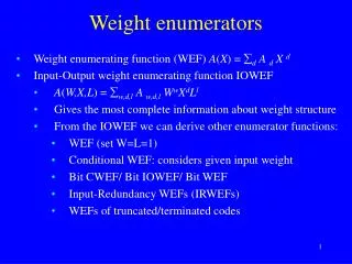
Weight enumerators. Weight enumerating function (WEF) A ( X ) = d A d X d Input-Output weight enumerating function IOWEF A ( W,X,L ) = w,d,l A w,d,l W w X d L l Gives the most complete information about weight structure From the IOWEF we can derive other enumerator functions:

Weight enumerators
E N D
Presentation Transcript
Weight enumerators • Weight enumerating function (WEF) A(X) = dAdXd • Input-Output weight enumerating function IOWEF • A(W,X,L) = w,d,lAw,d,lWwXdLl • Gives the most complete information about weight structure • From the IOWEF we can derive other enumerator functions: • WEF (set W=L=1) • Conditional WEF: considers given input weight • Bit CWEF/ Bit IOWEF/ Bit WEF • Input-Redundancy WEFs (IRWEFs) • WEFs of truncated/terminated codes
Conditional WEF • Aw(X) = dAw,dXd • …where Aw,d is the number of codewords of information weight w and code weight d • An encoder property • Useful for analyzing turbo codes with convolutional codes as component codes
Truncated/terminated encoders • Output length limited to = h + m blocks • h is the number of input blocks • m is the number of terminating output blocks (the tail) necessary to bring the encoder back to the initial state • For a terminated code, apply the following procedure: • Write the IOWEF A(W,X,L) in increasing order of L • Delete the terms of L degree larger than
Do we count all codewords? • No • Only those that start at time 0 • Why? • Each time instant is similar (for a time invariant code) • The Viterbi decoding algorithm (ML on trellis) makes decisions on k input bits at a time. Thus any error pattern will start at some time, and the error pattern will be structurally similar to an error starting at time 0 • Only first-event paths • Why? • Same as above • Thus FER/BER calculation depends on the first event errors that start at time 0
BER calculation • Bit CWEF Bw(X) = dBw,dXd • …where Bw,d= (w/k) Aw,d is the total number of nonzero information bits associated with all codewords of weight d and produced by information sequences of weight w, divided by k • Bit IOWEF B(W,X,L) = w,d,lBw,d,lWwXdLl • Bit WEF B(X) = dBdXd = w,dBw,dWwXd = w,d (w/k) Aw,dWwXd = 1/k(w,dwAw,dWwXd )/ W |W=1
IRWEF • Systematic encoders: codeword weight d = w + z, where z is the parity weight • This instead of the IOWEF A(W,X,L) = w,d,lAw,d,lWwXdLl, we may (and in some cases it is more convenient to) consider the input redundancy WEF A(W,Z,L) = w,z,lAw,z,lWwZzLl
Alternative to Mason’s formula • Introduce state variables i giving the weights of all paths from S0 to state Si • 1= WZL + L2 • 2= WL1+ ZL3 • 3= ZL1+ WL3 • A(W,Z,L) =WZL2 • Solve this set of linear equations
Distance properties • The decoding method determines what is actually the important distance property • The free distance of the code (ML decoding) • The column distance function (sequential decoding) • The minimum distance of the code (majority logic decoding)
Free distance • dfree = minu,u’ { d(v,v’) : u u’ } = minu,u’ { w(v+v’) : u u’ } = minu, { w(v) : u 0 } • Lowest power of X in the WEFs • Minimum weight of any path that diverge from the zero state and remerges later • Note: We implicitly assume noncatastrophic encoder here • Catastrophic encoders: May have paths of smaller weight than dfree that do not remerge
Column distance • [G]l : The binary matrix consisting of the first n(l+1) colums of G • Column distance function (CDF) dl : The minimum distance of the block code defined by [G]l • Important for sequential decoding
Special case of column distance • Special cases: • l=m, dl = minimum distance (important for majority logic decoding of convolutional codes) • l: dl dfree
Optimum decoding of CCs • A trellis offers an ”economic” representation of all codewords • Maximum likelihood decoding: The Viterbi algorithm • Decode to the nearest codewords • MAP decoding: The BCJR algorithm • Minimize information bit error probability • Turbo decoding applications
Trellises for convolutional codes • How to obtain the trellis from the state diagram • Make one copy of the states of a state diagram for each time instant • Let branches from states at time instant i go to states at time instant i+1
Example G(D) = [1 + D, 1+D2, 1+D+D2]
Metrics M(a,b) a b M(a,c) M(c,b) c that obeys the triangle inequality: M(a,b) M(a,c) + M(c,b) • A metric is a measure of (abstract) distance between (abstract) points
Metrics for a DMC Bit metrics:M(rj|vj) = logP(rj|vj) Branch metrics:M(rl|vl) = logP(rl|vl) Path metrics:M(r|v) = logP(r|v) • Information u = (u0,…, uh-1) = (u0,…, uK -1) K = kh • Codeword v = (v0,…, vh-1) = (v0,…, vN -1) N = n(h+m) • Receive r = (r0,…, rh-1) = (r0,…, rN -1) • Recall: • P(r|v) = l=0..h+m-1P(rl|vl) = j =0..N-1P(rj|vj) • ML decoder: Choose v to maximize this expression • …or to maximize log P(r|v) = l= 0..h+m-1logP(rl|vl) = j =0..N-1logP(rj|vj)
Partial path metrics • Path metric for the first t branches of a path • M([r|v]t) = l= 0..t-1M(rl|vl) = l= 0..t-1logP(rl|vl) = j =0..nt-1logP(rj|vj)
The Viterbi algorithm • Recursive algorithm to grow the partial path metric of the best paths going through each state. • Basic algorithm: • Initialize t=1. The loop of the algorithm looks like this: • (Add, Compare, Select) Add: Compute the partial path metrics for each path entering each state at time t, based on the partial path metrics at time t –1 and the branch metrics from time t-1 to time t.Compare all such incoming paths, and Select the (information block associated with the) best one, record its path gain and a pointer to where it came from. • t:=t+1. If t < h+m, repeat from 1. • Backtracing: At time h+m, Trace back through the pointers to obtain the winning path.
Proof of ML decoding • Theorem: The final survivor w in the Viterbi algorithm is an ML path, that is M(r|w) M(r|v), for all v C. • Proof: • Consider any non-surviving codeword v C • The paths v and w must merge in some state S at some time t • Since v was not the final survivor, it must have been eliminated in state S at time t • Thus M([r|w]t) M([r|v]t), and the best path from state S at time t to the terminal state at time h+m has a partial path metric not better than that of w • Alternative proof by recursion • The algorithm, finds the best path to each state at time1 • For t>0, if the algorithm finds the best path to each state at time t, it also the best path to each state at time t+1
Note on implementation (I) • In hardware!!! Implementations of the Viterbialgorithm often uses simple processors that either cannot process floating point numbers, or where such processing is slow • For a DMC the bit metrics can be represented by a finite size table • The bit metric M(rj|vj) = logP(rj|vj) is usually a real number, but • Since the algorithm only determines the path of maximum metric, the result is not affected by scaling or adding constants • Thus M(rj|vj) = logP(rj|vj) can be replaced by c2[logP(rj|vj)+c1] • Select the constants c1 and c2 such that all bit metrics values are closely approximated by an integer
Suggested exercises • 11.17-... • 12.1-12.5