Download

1 / 27
270 likes | 396 Views
Linear Programming An Example. Problem. The dairy "Fior di Latte" produces two types of cheese: cheese A and B. The dairy company must decide how many tons of each type of cheese can be produced. The company uses only the milk from some stables that can provide 2880 tons of milk per year.

E N D
Linear Programming An Example
Problem The dairy "Fior di Latte" produces two types of cheese: cheese A and B. The dairy company must decide how many tons of each type of cheese can be produced. The company uses only the milk from some stables that can provide 2880 tons of milk per year. From the processing point of view, the two cheeses differ in the amount of milk and in the work needed to produce one unit of processed product In fact, 1 ton of A cheese requires 12 tons of milk and 9 hours of work, while, 1 ton of B needs 16 tons of milk and 6 hours of work. The dairy has a maximum capacity of 200 tons of cheese. The hours available are 1566. The profit that the company can benefit from cheese sale is 350 euros for cheese A and 300 euros for cheese B. The question is: how many tons of cheese A and B the company should produce in order to obtain the maximum profit?
Problems of choice In any economic context where resources to be used are available in limited quantities, there is a problem of choice concerning the quantities and combinations of factors to be used to obtain the best possible result. For example, entrepreneurial activity has as main purpose the continuity of their business and the factors of production remuneration. The entrepreneur organizes his activities in order to find that combination of factors that can provide the highest profit. In the field of transport logistics, for example, the goal is to find the shortest way to reach a certain place to minimize the transport costs of goods.
Developing the problem To solve any linear programming problem, first of all we must try to formulate it in algebraic terms by following these rules: 1. Understanding the problem; 2. Identify the decision variables; 3. Identify the objective function as a linear combination of decision variables; 4. Formulate the constraints of the problem as a linear combination of decision variables.
Understanding the problem Before dealing with the mathematical formulation of each problem , it is important to consider the context in which we are developing a mathematical programming model and ask to ourselves: 1. Which is the goal to which we respond by developing a mathematical programming model? 2. There are decision variables that can influence the objective? 3. Which are the factors or resources used in the technical-economic transformation process? 4. Which are the times required to give a decision support? 5. It 's really necessary to develop a mathematical programming model?
Identifying the decision variables If we have understood the terms of the problem, then we can identify the decision variables, those variables that through the use of the resources available in limited quantities determine the outcomes of the problem. The variables are those elements of the problem that have to be calculated to obtain the best possible result. Usually the variables of a LP problem are identified by the letters X1, X2, X3, … , Xn In our example, the decision variables are implicit in the final question: how many tons of cheese A and B the company should produce to maximize profit? The variables are: Cheese A X1 Decision variables for the LP problem Cheese B X2
Objective Function After having identified the decision variables of the problem, we formulate in mathematical terms the objective of the LP problem . Question: What is to be maximized / minimized? The objective function is the algebraic transposition of the aim of who want to optimize a given situation using a LP model. In our example, the objective function is given by maximizing the total profit of the dairy, namely: Total Profit = 350 X1 + 300 X2 Objective= maximize (max) Total Profit Objective Function= max Total Profit = max 350 X1 + 300 X2
Constraints In each choice issue, there are bounds to the values that decision variables can assume. In particular, in each of LP problem it is very important to consider the limiting factors, namely the resources available in limited quantities. Moreover, in many problems of choice it is necessary to consider the technological constraints, namely the links between variables and between variables and limiting factors. In the LP problem we considerd we can see 3 main constraints. I constraint. The dairy wearhouse capacity The dairy can contain up to 200 tons of cheese. In other terms: X1 + X2≤ 200 The quantity of cheese A added to the quantity of cheese B cannot be higher that 200 tons.
Constraints II constraint. The technological constraint on the milk availibility The dairy company uses milk produced by some breeders to make the two types of cheese: 12X1 + 16X2≤ 2880 To produce one unit (ton) of cheese A it is necessary to use 12 tons of milk and to produce cheese B It needs to use 16 tons of milk. The total amount of milk that may enter in the dairy processing is equal to 2880 tons. III constraint. The constraint on work The maximum amount of hours that can be devoted to the processing activity represents a further constraint to the problem. In fact: 9X1 + 6X2≤ 1566 9 hours to produce 1 ton of cheese A and 6 hours to produce 1 ton of cheese B.
Constraints Finally, to achieve consistency between the solutions of the problem with the observed reality and in order to avoid implausible solutions to LP problems, the so-called non-negativity constraints related to variables must be added. So in our example, it would be surprising to obtain solutions with negative values of decision variables. For this reason, the problem is integrated by the following 2 constraints: X1 ≥ 0 Non-negativity constraints X2 ≥ 0 The two constraints ensure that the solution of the problem be realistic and coherent.
The LP Problem Now, we can write the LP problem in its full algebraic formulation: Objective Function Subject to Dairy capacity Milk supply Labour availibility Non-negativity 1 Non-negativity 2 Activity 1 Activity 2
Graphical Solution The constraints of a LP problem define the set of feasible solutions, i.e. the region of feasible solutions for the problem (feasible region). Our task is to determine which point of the feasible region corresponds to the optimal value of the objective function. Subject to
Graphical Solution Let us represent the first constraint x2 (0,200) 200 150 100 50 (200,0) x1 0 50 100 150 200
Graphical Solution Let us represent the first constraint x2 (0,200) 200 Boundary line for the dairy company capacity 150 100 50 (200,0) x1 0 50 100 150 200
Graphical Solution Let us represent the first constraint x2 250 (0,180) 200 Boundary line for the dairy company capacity 150 100 50 (240,0) x1 0 50 100 150 200 250
Graphical Solution Let us represent the second constraint x2 250 (0,180) 200 Boundary line for the milk supply 150 100 50 (240,0) x1 0 50 100 150 200 250
Graphical Solution Let us represent the third constraint x2 (0,261) 250 200 Boundary line for the avaiable labour hours 150 100 50 (174,0) x1 0 50 100 150 200 250
Graphical Solution Let us represent the third constraint x2 (0,261) 250 200 Boundary line for the avaiable labour hours 150 100 Feasible region 50 (174,0) x1 0 50 100 150 200 250
Graphical Solution The feasible region is the cloud of points with respect to which the values assumed by the decision variables do not conflict with the constraints of the problem. x2 250 200 Feasible Region 150 100 50 x1 0 50 100 150 200 250
Graphical Solution The feasible region offers an endless cloud of points in which we find the pair of valuesthat produce the highest profit. For this reason, there is an infinite number of values of the objective function that satisfies the constraints of the problem. However, only a point allows to get the maximum value of the objective function. The research of this point shall follow the criterion of saturation of the limited factors. You must find the solution that fully utilizes the scarce resources. This is why, the solution of our problem must be found on the border line of the feasible region. In LP, these points are in correspondence of the intersection of the constraint lines, namely the corner points of the feasible region.
Graphical Solution We proceed by trial from the following value of the objective function: 350x1 + 300x2 = 35000 Graphically: x2 250 200 Objective Function 150 (0,116.67) 100 50 (100,0) x1 0 50 100 150 200 250
Graphical Solution The objective function value satisfies the previous constraints, but it does not maximize the result because we still have availability factors to use. Let us now with an OF value equal to 52500 euro. Graphically: x2 250 200 (0,175) New objective function 150 100 50 (150,0) x1 0 50 100 150 200 250
Graphical Solution By moving the objective function at the extremes of the feasible region, the economic performance continues to increase. The point beyond which no longer can move the OF is the optimal point. x2 250 200 150 Optimal solution (122,78) 100 50 x1 0 50 100 150 200 250
Graphical Solution To find the optimal solution of a LP problem it is necessary to study the corner points and determine the value of the objective function. The point that returns the highest value of OF coincides with the optimal point. x2 250 (0,180) OF=54000€ 200 (80,120) OF=64000€ 150 (122,78) OF=66100€ 100 50 (174,0) OF=60900€ (0,0) OF=0€ x1 0 50 100 150 200 250
LP Problem Solve graphically the following LP problem. Subject to
Graphical Solution Some problems may present multiple optimal solutions x2 250 (0,180) OF=54000€ 200 (80,120) OF=72000€ 150 (122,78) OF=78300€ 100 50 (174,0) OF=78300€ (0,0) OF=0€ x1 0 50 100 150 200 250
LP Problem Solve graphically the following LP problem: Subject to