Download
1 / 23
230 likes | 388 Views
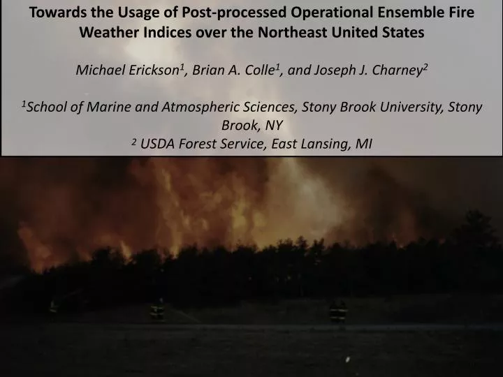
Towards the Usage of Post-processed Operational Ensemble Fire Weather Indices over the Northeast United States Michael Erickson 1 , Brian A. Colle 1 , and Joseph J. Charney 2 1 School of Marine and Atmospheric Sciences, Stony Brook University, Stony Brook, NY

E N D
Towards the Usage of Post-processed Operational Ensemble Fire Weather Indices over the Northeast United States Michael Erickson1, Brian A. Colle1, and Joseph J. Charney2 1School of Marine and Atmospheric Sciences, Stony Brook University, Stony Brook, NY 2USDA Forest Service, East Lansing, MI
Ridge-Manorville Brush Fire – April 9th, 2012 • 1000-2000 acres burned. • 600 firefighters from 109 departments battled the fire with 30 brush trucks, 20 tankers and 100 engines. • New York State Police Helicopters made airdrops of water. • Fortunately the fire broke out in a relatively rural area of Long Island. Source: longislandpress.com Source: new12.com Source: newsday.com
Sunrise Fire – late August 1995 • 7000 acres burned by a series of brush fires between late August and early September. • Highways and railways were closed cutting off the Hamptons from the rest of Long Island. • Numerous homes and business were damaged, as was the pine barrens ecosystem. Source: pb.state.ny.us Source: pb.state.ny.us Source: dmna.ny.gov
How well do operational models perform on days where the atmosphere is mild, dry, and windy? • A near-surface weather based fire threat index could have potential utility for fire weather forecasters, particularly if some post-processing is involved. • The proliferation of ensemble atmospheric forecasting should be utilized to create fire threat forecasts. Motivation Goals • Define a High Fire Threat Weather Index (HFTWI) that captures the occurrence and strength of fire risk. • Explore the climatology of HFTWI for the New York City tri-state region. • Evaluate the accuracy of atmospheric ensembles in predicting high fire threat and determine if any deficiencies/biases can be corrected. • Propose methods for how post-processing and probabilistic methods can be used to maximize the accuracy of ensemble high fire threat forecasts.
Dry conditions are a necessary condition for the development and spread of fires in the Northeast United States. • Strong winds are then important to spread the fires and make them large. • Fire threat should be evaluated over a region to increase sample size but of relatively small size to ensure that the weather experienced is homogenous. Defining High Fire Threat Weather Index (HFTWI) - Assumptions Source: longislandpress.com
Uses Automated Surface Observing System (ASOS) station observations between 1979-2012. • No rainfall > 0.5” or snow cover can occur at any station 24 hours before the high fire threat day starts. • HFTWI consists of 5 categories; 3 from relative humidity (RH) and 2 from wind speed (WS). • The hourly RH must be in the bottom 2, 1, and 0.5 percentile to achieve sub-categories 1, 2, and 3, respectively. • If RH criteria is meet, WS in the top 75 and 95 percentile is needed to meet WS criteria for sub-categories 1 and 2, respectively. • HFTWI is the sum of the RH and WS components and varies between 0 and 5. • HFTWI computed for all stations/hours separately. Daily HFTWI uses the station median of the daily maximum values. High Fire Threat Weather Index (HFTWI)- Definition RH Hourly Histogram Arrows indicate bottom 0.5, 1, and 2.0 percentile, respectively
Fire Threat Frequency by Month Fire Threat Frequency by Year Fire Threat Frequency by Month HFTWI Climatology– Monthly and Annual Variability
Fire Threat – Monthly and Annual Variability • Verified the National Center For Environmental Prediction (NCEP) Short Range Ensemble Forecast (SREF) system from 3/6/2006-6/30/2012. • Since METAR observations can not be used to verify gridded products, the Rapid Update Cycle (RUC) analyses are used as verification. • Model bias and error are represented by computing mean error (ME) and mean absolute error (MAE) for each HFTWI category. Methods and Data Region of Study 09 UTC NCEP SREF 21 Member Ensemble • Consists of 4 different models: • The old Eta model. • The Regional Spectral Model (RSM). • The Weather Research & Forecasting (WRF) Advanced Research WRF (ARW). • The WRF Non-hydrostatic Mesoscale Model (NMM).
Comparing RUC and METAR – Bias and MAE • Before verifying the SREF ensemble against the RUC, the RUC should be compared to “real” METAR observations. • In this case, the RUC data is bilinearly interpolated to the METAR observations. • For simplicity, the HFTWI rather than individual variables are verified. • On the average, the RUC has a small positive bias in HFTWI compared to observations. • The MAE varies from about 1.5 categories at low thresholds to slightly over 2 categories of HTWFI at high thresholds.
Comparing RUC and METAR - Biases Urban Coast Long Island Inland AM PM (UTC) • RUC and METAR observations compute similar HFTWI values. However the RUC overestimates (underestimates) HFTWI during the morning (afternoon).
HFTWI • Gridded HFWTI is the same for RUC/SREF as METAR observations, with the following exceptions: • HFTWI computed for each grid point rather than for each station. • The stage IV precipitation data set is used to determine recent rainfall while the Multisensor Snow and Ice Mapping System (IMS) Northern Hemisphere Snow and Ice Analysis is used to find snow cover. • Haines Index • Derived solely from the lapse rate and dew-point depression of the lower atmosphere. The exact vertical level depends on the surface elevation. • Computed for each grid point like HFTWI and split into three elevation categories 1) below 200 m, 2) between 200 m and 1000 m, and 3) above 1000 m. • All verifying RUC data is bilinearly interpolated to the SREF domain . Adaption of High Fire Threat Metrics to Gridded Datasets
Observed HFTI Versus Ensemble mean HFTWI Example from 4/7/2012 0900 UTC SREF Run RUC “Observed” HFTWI SREF Ensemble Mean HFTWI
Model Verification and Post-Processing Details Region of Study High Fire Threat Day Classification • A high fire threat day is considered to have a domain averaged HFTWI of 1 or greater. This is determined by taking the spatial median of each sites daily maximum HFTWI. • Model verification is performed for all high fire threat days determined from the RUC analysis. Bias Correction Details • A running-mean bias correction (Wilson et al. 2007) is used to bias correct 2-m temperature as in Erickson et al. (2012). • The previous 14 high fire threat days are used for bias correction.
Ensemble Haines Index Verification - Bias PM AM PM AM PM AM Model Hour • The SREF under predicts the Haines index with the RSM core having the greatest negative bias. Bias correction is effective on the average.
Ensemble Haines Index Verification– MAE MAE PM AM PM AM PM AM • MAE reflects the under prediction of the Haines Index from the SREF. Bias correction improves MAE by hour and model core in most cases.
Ensemble Haines Index Verification– Breakdown by Variable • The under prediction of the Haines Index is caused by the model being too cool and moist, particularly in the lower levels.
Ensemble HFTWI Verification - Bias PM AM PM AM PM AM • The under prediction of the HFTWI by the NCEP SREF is quite drastic, although bias correction adjusts this under prediction rather well.
Ensemble HFTWI Verification– MAE PM AM PM AM PM AM MAE PM AM PM AM PM AM • As with the Haines Index, bias correction improves MAE over the raw HFTWI in most cases.
Ensemble HFTWI Verification– Breakdown by Variable • The bias in HFTWI is caused by the SREF having too much low level moisture during high fire threat days.
A new fire metric called the High Fire Threat Weather Index (HFTWI) has been developed which solely considers low level atmospheric parameters. This can be used on model forecast grids operationally by fire meteorologists. • The climatology of HFTWI between 1979-2012 reveals a strong peak in fire threat risk between March and May and has been increasing in frequency slightly in recent years. • Verifying both the Haines and HFTWI forecasts calculated from the NCEP SREF ensemble reveal a persistent under prediction of both indices compared to RUC analyses. This is caused by the low levels of the model being both too cool and too wet. • A simple bias correction that considers previous high fire threat days on average reduces the bias and mean absolute error of both the Haines Index and HFTWI. Further research is needed to adapt an analog fire-related bias correction operationally. • Future work will utilize probabilistic forecasts of high fire threat. For operational examples see: http://foggy.somas.stonybrook.edu/fire/ Conclusions