Download
1 / 17
170 likes | 339 Views
ESTIMATING THE REGRESSION COEFFICIENTS FOR SIMPLE LINEAR REGRESSION. Step 2: Estimating β 1 and β 0. In simple linear regression, in Step 1, it was hypothesized that: y = 0 + 1 x + In Step 2, the best estimates for 0 and 1 are determined.

E N D
ESTIMATING THE REGRESSION COEFFICIENTS FOR SIMPLE LINEAR REGRESSION
Step 2: Estimating β1 and β0 • In simple linear regression, in Step 1, it was hypothesized that: y = 0 + 1x + • In Step 2, the best estimates for 0and 1are determined. • These “best estimates” are designated as b0 and b1 respectively.
DETERMINING THE BEST STRAIGHT LINE • The best straight line is the one that, in some sense, minimizes the overall errors. • But the positive values for the errors will offset the negative values giving an average error value of 0. • To make sure all quantities are positive -- the errors are squared. • THE BEST STRAIGHT LINE MINIMIZES THE SUM OF THE SQUARED ERROR (SSE)
MINIMIZING SSE • We want to minimize SSE where: This is a function in two variables: b0 and b1.
Method of Least Squares • Because we are minimizing the sum of the squared errors, the approach for doing this is called the METHOD OF LEAST SQUARES. • To find the minimum of a function of two variables (b0 and b1), take partial derivatives with respect to each of the variables and set them equal to 0. • We then have two equations in the two unknowns and we can solve for the values of the two unknowns -- these are known as the NORMAL EQUATIONS for regression.
THE PARTIAL DERIVATIVES The result from taking the partial derivatives of SSE and setting them equal to 0 is: Simplifying gives the two normal equations for b0 and b1:
SOLVING FOR b1THE BEST ESTIMATE FOR 1 Solving the normal equations for b1 gives: Doing a little algebra, gives these three alternate formulas:
SOLVING FOR b0THE BEST ESTIMATE FOR β0 Regardless of how b1 is calculated, b0 is found by: And the regression equation is:
Example – The Data SUM 9400 959000
Example – Table Calculations SUM 23,340,000 444,000
CALCULATING b1 AND b0THE REGRESSION EQUATION Thus the estimated regression equation is:
What does the model predict sales to be when $1150 is spent on advertising? What does the model predict sales to be when $5,000,000 is spent on advertising? But $5,000,000 is way outside the observed values for x. The model should not be used for such predictions.
Choose Regression from Data Analysis By EXCEL
Location of Y-values X-values Output Worksheet Check Labels
b0 b1 Regression Equation Y = 46486.49 + 52.56757x
Review • b0, the point estimate for 0 , and b1, the point estimate for 1, are found from calculus by minimizing the total sum of the squared errorsbetween the actual and predicted values of y. • The regression equation coefficients can be found by Excel or by hand by: • The regression equation should not be used for values of x that are “far away” from the observed x values.