Download

1 / 38
391 likes | 613 Views
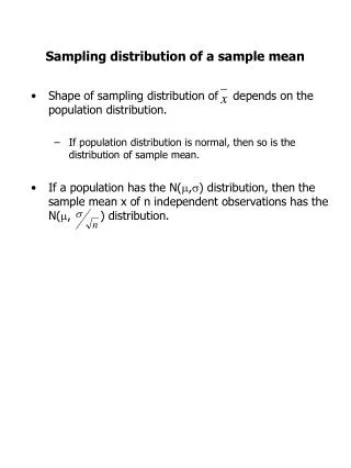
Sampling Distribution of a Sample Proportion. Lecture 25 Sections 8.1 – 8.2 Fri, Feb 29, 2008. Sampling Distributions. Sampling Distribution of a Statistic. The Sample Proportion. The letter p represents the population proportion .

E N D
Sampling Distribution of a Sample Proportion Lecture 25 Sections 8.1 – 8.2 Fri, Feb 29, 2008
Sampling Distributions • Sampling Distribution of a Statistic
The Sample Proportion • The letter p represents the population proportion. • The symbol p^ (“p-hat”) represents the sample proportion. • p^ is a random variable. • The sampling distribution of p^ is the probability distribution of all the possible values of p^.
Example • Suppose that 2/3 of all males wash their hands after using a public restroom. • Suppose that we take a sample of 1 male. • Find the sampling distribution of p^.
W P(W) = 2/3 2/3 1/3 N P(N) = 1/3 Example
Example • Let x be the sample number of males who wash. • The probability distribution of x is
Example • Let p^ be the sampleproportion of males who wash. (p^ = x/n.) • The sampling distribution of p^ is
Example • Now we take a sample of 2 males, sampling with replacement. • Find the sampling distribution of p^.
W P(WW) = 4/9 2/3 W 1/3 2/3 N P(WN) = 2/9 1/3 W P(NW) = 2/9 2/3 N 1/3 N P(NN) = 1/9 Example
Example • Let x be the sample number of males who wash. • The probability distribution of x is
Example • Let p^ be the sampleproportion of males who wash. (p^ = x/n.) • The sampling distribution of p^ is
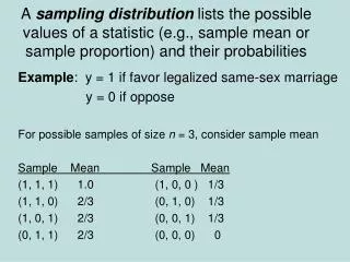
Samples of Size n = 3 • If we sample 3 males, then the sample proportion of males who wash has the following distribution.
Samples of Size n = 4 • If we sample 4 males, then the sample proportion of males who wash has the following distribution.
Samples of Size n = 5 • If we sample 5 males, then the sample proportion of males who wash has the following distribution.
Our Experiment • In our experiment, we had 80 samples of size 5. • Based on the sampling distribution when n = 5, we would expect the following
The pdf when n = 2 0 1/2 1
The pdf when n = 3 0 1/3 2/3 1
The pdf when n = 4 0 1/4 2/4 3/4 1
The pdf when n = 5 4/5 0 1/5 2/5 3/5 1
The pdf when n = 10 8/10 0 2/10 4/10 6/10 1
Observations and Conclusions • Observation: The values of p^ are clustered around p. • Conclusion:p^ is close to p most of the time.
Observations and Conclusions • Observation: As the sample size increases, the clustering becomes tighter. • Conclusion: Larger samples give better estimates. • Conclusion: We can make the estimates of p as good as we want, provided we make the sample size large enough.
Observations and Conclusions • Observation: The distribution of p^ appears to be approximately normal. • Conclusion: We can use the normal distribution to calculate just how close to p we can expect p^ to be.
One More Observation • However, we must know the values of and for the distribution of p^. • That is, we have to quantify the sampling distribution of p^.
The Central Limit Theorem for Proportions • It turns out that the sampling distribution of p^ is approximately normal with the following parameters.
The Central Limit Theorem for Proportions • The approximation to the normal distribution is excellent if
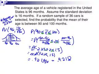
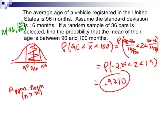
Example • If we gather a sample of 100 males, how likely is it that between 60 and 70 of them, inclusive, wash their hands after using a public restroom? • This is the same as asking the likelihood that 0.60 p^ 0.70.
Example • Use p = 0.66. • Check that • np = 100(0.66) = 66 > 5, • n(1 – p) = 100(0.34) = 34 > 5. • Then p^ has a normal distribution with
Example • So P(0.60 p^ 0.70) = normalcdf(.60,.70,.66,.04737) = 0.6981.
Why Surveys Work • Suppose that we are trying to estimate the proportion of the male population who wash their hands after using a public restroom. • Suppose the true proportion is 66%. • If we survey a random sample of 1000 people, how likely is it that our error will be no greater than 5%?
Why Surveys Work • Now we have
Why Surveys Work • Now find the probability that p^ is between 0.61 and 0.71: normalcdf(.61, .71, .66, .01498) = 0.9992. • It is virtually certain that our estimate will be within 5% of 66%.
Case Study • Study confirms aprotinin drug increases cardiac surgery death rate • Aprotinin during Coronary-Artery Bypass Grafting and Risk of Death
Why Surveys Work • What if we had decided to save money and surveyed only 100 people? • If it is important to be within 5% of the correct value, is it worth it to survey 1000 people instead of only 100 people?
Quality Control • A company will accept a shipment of components if there is no strong evidence that more than 5% of them are defective. • H0: 5% of the parts are defective. • H1: More than 5% of the parts are defective.
Quality Control • They will take a random sample of 100 parts and test them. If no more than 10 of them are defective, they will accept the shipment. • What is ? • What is ?