Download
1 / 18
180 likes | 428 Views
Semi-Supervised Classification by Low Density Separation. Olivier Chapelle, Alexander Zien. Student: Ran Chang. Introduction. Goal of semi-supervised classification: Use unlabeled data to improve the generalization Cluster assumption:

E N D
Semi-Supervised Classification by Low Density Separation Olivier Chapelle, Alexander Zien Student: Ran Chang
Introduction • Goal of semi-supervised classification: Use unlabeled data to improve the generalization • Cluster assumption: The decision boundary should not cross high density regions, but instead lie in low density regions
Algorithm • N labeled data points • M unlabeled data points • Labels
Graph-based similarities (cont) • Principle: Assign low similarities to pairs of points that lie in different clusters • If two points in same cluster: exit a continuous connecting curve that only goes through regions of high density • If two points in different clusters: such curve has to traverse a density valley. • Definition of similarity of 2 points: maximizing over all continuous connecting curves the minimum density along the connection
Graph-based similarities (cont) • Build nearest neighbor graph G from all (labeled and unlabeled) data. • Compute the n x (n + m) distance matrix of minimal -path distances according to from all labeled points to all points
Graph-based similarities (cont) 3. Perform a non-linear transformation on to get kernel K 4. Train a SVM with K and predict
Graph-based similarities (cont) • Usage of p: the accuracy of this approximation depends on the value of the softening parameter p: for p -> 0, the direct connection is always shortest, so that every deletion of an edge can cause the corresponding distance to increase; for p->infinity, shortest paths almost never contain any long edge, so that edges can safely be deleted. • For large values of p, the distance between points in the same cluster are decreased; in contrast, the distances between points from different clusters are still dominated by the gaps between the clusters.
Gradient TSVM • The last term make this problem non-convex and it is not differentiable. So we replace it by
Gradient TSVM (cont) • initially set C* to a small value and increase it exponentionally to C • The choice of setting the final value of C* to C is somewhat arbitrary. Ideally, it would be preferable to consider this value as a free parameter of the algorithm.
Multidimensional Scaling (MDS) • Reason: The derived kernel is not positive definite. • Goal: Find a Euclidean embedding of before applying Gradient TSVM.
Experiment • Data Sets • g50c and g10n are from two standard normal multi-variant Gaussians. • g50c: the labels correspond to the Gaussians, and the means are located in 50-dimensional space such that the Bayes error is 5% • Similarly, g10n is in 10 dimensions • Coil20:gray-scale images of 20 different objects taken from different angles, in steps of 5 degrees • Text: the classes mac and mswindows of the Newsgroup20 dataset preprocessed. • Uspst: data part of the well-known USPS data on handwritten digit recognition.
Appendix (Dijkstra algorithm) • Dijkstra's algorithm is known to be a good algorithm to find a shortest path. • Set i=0, S0= {u0=s}, L(u0)=0, and L(v)=infinity for v <> u0. If |V| = 1 then stop, otherwise go to step 2. • For each v in V\Si, replace L(v) by min{L(v), L(ui)+dvui}. If L(v) is replaced, put a label (L(v), ui) on v. • Find a vertex v which minimizes {L(v): v in V\Si}, say ui+1. • Let Si+1 = Si cup {ui+1}. • Replace i by i+1. If i=|V|-1 then stop, otherwise go to step 2.