Download
1 / 28
330 likes | 968 Views
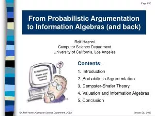
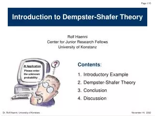
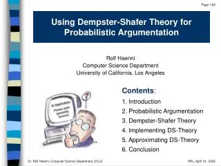
Using Dempster-Shafer Theory for Probabilistic Argumentation. Rolf Haenni Computer Science Department University of California, Los Angeles. Contents :. 1. Introduction 2. Probabilistic Argumentation 3. Dempster-Shafer Theory 4. Implementing DS-Theory 5. Approximating DS-Theory

E N D
Using Dempster-Shafer Theory for Probabilistic Argumentation Rolf Haenni Computer Science DepartmentUniversity of California, Los Angeles Contents: 1. Introduction 2. Probabilistic Argumentation 3. Dempster-Shafer Theory 4. Implementing DS-Theory 5. Approximating DS-Theory 6. Conclusion
Cons Pros 1. Introduction Reasoning and deciding under uncertainty is common in everyone’s daily life: 1) elaborate possible answers or alternatives 2) list pros and cons (for each answer or alternative) 3) measure or weigh pros and cons (for each answer or alternative) 4) acceptanswer or choose alternative with the maximal total weight (or gather more information, if necessary)
The most popular formal approach is different: 1) elaborate possible answers or alternatives 2) build probabilistic model (usually a Bayesian network) 3) compute posterior probabilities (for each answer or alternative) 4) apply decision theory (maximize expected utility or minimize expected cost) This disrespects: 1) the true nature of uncertain reasoning observed in everyone’s daily life 2) the existence of partial or total ignorance e.g. knowing that p(head)=0.5 is different than not knowing the probability p(head)
p(e|c) = 0.2 p(c) = 0.1 p(e|c) = 0.7 C E p(e|c) = 0.8 p(c) = 0.9 p(e|c) = 0.3 p(e) = 0.1*0.7 + 0.9*0.2 = 0.25 p(e) = 0.1*0.3 + 0.9*0.8 = 0.75 e a1c p(a1)=0.1 0.1: c a1a2 a1c p(a2)=0.7 0.9: c a1a3 a2 (c e) p(a3)=0.2 0.7: c e a2 (c e) e 0.3: c e a3 (c e) a1a2 0.2: c e a3 (c e) a1a3 0.8: c e 2. Probabilistic Argumentation
1. Modeling Knowledge Uncertain Knowledge p(a) R a®R Fact: p(a) a® (R ® S) R ® S Simple Rule: p(a) a® General Rule: More general: Most general: Ingredients: • propositions • assumptions • prop. formulas - possible states - risk elements - interpretations - unknown circumst. - uncertain outcomes - measurement errors
2. Qualitative Analysis arguments pro/contra Hypothesis hypothesis open question about unknownor future world a) arguments in favor of combination of assumptions proving the hypothesis b) counter-arguments against combination of assumptions disproving the hypothesis Example: a1®X a4 a1 a2 arguments (a2a3) ®Y hypothesis knowledgebase a1a3 (XY) ®Z Z a2 a5 a4®Z counter-arguments a3 a5 (a5Y) ®Z
3. Quantitative Analysis a) define probability distributionover e.g. independent probabilities p(ai) for each assumption b) compute degree of support: conditional probability that at least one argument is true (given no conflicts) c) compute degree of possibility: one minus conditional probability that at least one counter-argument is true (given no conflicts) Remarks: 1) 2) support is sub-additive: 3) possibility is super-additive: 4) support and possibility are non-monotone! 5) and means total ignorance
Remark: Every probabilistic argumentation system can be trans-formed into a set of Dempster-Shafer belief potentials such that and for all AnytimeAlgorithm Degree ofSupport Arguments Belief Probabilistic ArgumentationSystem Dempster-Shafer BeliefPotentials Hypothesis Hypothesis Degree ofPossibility Counter-Arguments Plausibility
Y Additive: H E X Sub-additive: Z H Y E X J. Bernoulli: “Ars Conjectandi”, 1713 3. Dempster-Shafer Theory
1. Modeling a) define variables, domains, and frames with b) define belief potentials (mass functions) with Knowledge base: 2. Quantitative Analysis: (sub-additive) belief: plausibility: (super-additive)
632 binary variables • 1118 belief potentials with • 1117 combinations, 630 variables to eliminate • binary join tree with 2235 nodes 2 focal sets Example:
Exact computation: 3,320,390 ms (~56 minutes) Approximation: Error <1% after 60 seconds
Combination: Marginalization: intersection: projection: 4 crucial operations extension: equality testing: 4. Implementing DS-Theory
2) Bit strings very good for small domains • very fast intersection and equality testing • expensive projection and extension • high memory consumption for large domains 3) Logical representations: a) DNF’s intersection and equality testing is expensive b) CNF’s projection and equality testing is expensive c) OBDD’s not studied so far (all four crucial operations can be done in polynomial time) Representing Focal Sets: 1) List of vectors beyond practical applicability
with Example: Remarks: - - size of bit strings depends exponentially on the domain size Bit String Representation:
Combination: • intersect focal sets pair-wise and multiply their masses • regroup equal sets and sum over the masses Marginalization: • project focal sets • regroup equal sets and sum over the masses Approaches: 1) Simple lists beyond practical applicability 2) Ordered lists beyond practical applicability 3) Binary trees good (with exceptions) 4) AVL trees generally good 5) Hash tables generally good (better than AVL trees) Regrouping:
Quasi-Projection: Fusion: Remark: Many intersections are equal, and as a consequence, their projections are equal, too. use memoizing (store previous results in hash table)
Architectures: (A1) Classical method (combination followed by marginalization) (A2) Step-wise marginalization (combination followed by step-wise variable elimination) (A3) Fusion: a) without memoizing b) with memoizing Experiments:
1430 focal sets (largest mass: 0.452; smallest mass: 0.349*10-22) 5. Approximating DS-Theory
Incomplete Belief Potentials: Degree of incompleteness: Completeness relation: “ is less complete than “ partial order (reflexive, anti-symmetric, transitive)
Theorem 1: (unnormalized belief) Theorem 2: (unnormalized plausibility)
Normalized degree of incompleteness: Theorem 3: (normalized belief) Theorem 4: (normalized plausibility)
Theorem 5: (combination preserves incompleteness) Theorem 6: (marginalization preserves incompleteness) Remark: Incomplete belief potentials are obtained by removing focal sets with small masses: (only the k highest masses are kept)
Example: • computation often infeasible • effective running time is not predictable
with Such a time-dependent combination operator can be defined for belief potentials as an incremental procedure that starts with intersecting the highest masses first and stops when the time is over. Remark: Resource-bounded combination:
Problem: choose parameters t during propagation (if the total time is restricted to T milliseconds) Solution: share T equally among the nodes of the join tree and redistribute unused portions Example: T = 100 s = 5
Remarks: • the result of the procedure is an approximation of the exact computation: , • the procedure stops after at most T milliseconds • the method relies on the assumption that the time for marginalization is negligible • the same idea can be used for the outward propagation phase • a refining procedure exists for cases where the accuracy of the results is not satisfactory (this leads to convenient anytime algorithms)
5. Conclusion • Probabilistic argumentation is a natural approach to reasoning under uncertainty • Quantitative queries can be solved using DS-theory • Important tools for implementing DS-theory are: bit strings, hash tables, quasi-projection, fusion, and memoizing • Incomplete belief potentials allow to approximate belief and plausibility by lower and upper bounds • The resource-bounded combination operator allows to define inward and outward propagation as a resource-bounded procedure • Idea can be generalized for valuation algebras (axioms)