Download
1 / 30
310 likes | 504 Views
Nonlinear and Non-Gaussian Estimation with A Focus on Particle Filters. Prasanth Jeevan Mary Knox May 12, 2006. Background. Optimal linear filters Wiener Stationary Kalman Gaussian Posterior, p(x|y) Filters for nonlinear systems Extended Kalman Particle.

E N D
Nonlinear and Non-Gaussian Estimation with A Focus on Particle Filters Prasanth Jeevan Mary Knox May 12, 2006
Background • Optimal linear filters • Wiener Stationary • Kalman Gaussian Posterior, p(x|y) • Filters for nonlinear systems • Extended Kalman • Particle
Extended Kalman Filter (EKF) • Locally linearize the non-linear functions • Assume p(xk|y1,…,k) is Gaussian
Particle Filter (PF) • Weighted point mass or “particle” representation of possibly intractable posterior probability density functions, p(x|y) • Estimates recursively in time allowing for online calculations • Attempts to place particles in important regions of the posterior pdf • O(N) complexity on number of particles
Particle Filter Background [Ristic et. al. 2004] • Monte Carlo Estimation • Pick N>>1 “particles” with distribution p(x) Assumption: xi is independent
Importance Sampling • Cannot sample directly from p(x) • Instead sample from known importance density, q(x), where: • Estimate I from samples and importance weights where
Sequential Importance Sampling (SIS) • Iteratively represent posterior density function by random samples with associated weights Assumptions: xk Hidden Markov process, yk conditionally independent given xk
Degeneracy • Variance of sample weights increases with time if importance density not optimal [Doucet 2000] • In a few cycles all but one particle will have negligible weights • PF will updating particles that contribute little in approximating the posterior • Neff, estimate of effective sample size [Kong et. al. 1994]:
Optimal Importance Density [Doucet et. al. 2000] • Minimizes variance of importance weights to prevent degeneracy • Rarely possible to obtain, instead often use
Resampling • Generate new set of samples from: • Weights are equal after i.i.d. sampling • O(N) complexity • Coupled with SIS, these are the two key components of a PF
Sample Impoverishment • Set of particles with low diversity • Particles with high weights are selected more often
Sampling Importance Resampling (SIR)[Gordon et. al. 1993] • Importance density is the transitional prior • Resampling at every time step
SIR Pros and Cons • Pro: importance density and weight updates are easy to evaluate • Con: Observations not used when transitioning state to next time step
Auxiliary SIR - Motivation[Pitt and Shephard 1999] • Want to use observation when exploring the state space ( ’s) • To have particles in regions of high likelihood • Incorporate into resampling at time k-1 • Looking one step ahead to choose particles
ASIR - from SIR • From SIR we had • If we move the likelihood inside we get: • We don’t have though • Use , a characterization of given • such as
ASIR continued • So then we get: • And the new importance weight becomes:
ASIR Pros & Cons • Pro • Can be less sensitive to peaked likelihoods and outliers by using observation • Outliers - Model-improbable states that can result in a dramatic loss of high-weight particles • Cons • Added computation per cycle • If is a bad characterization of (ie. large process noise), then resampling suffers, and performance can degrade
Simulation Linear • System Equations: where v ~ N(0,6) and w ~ N(0,5)
Simulation Linear Table 1: Mean Squared Error Per Time Step
Simulation Nonlinear • System Equations: where v ~ N(0,6) and w ~ N(0,5)
Simulation Nonlinear Table 2: Mean Squared Error Per Time Step
Conclusion • PF approaches KF optimal estimates as N • PF better than EKF for nonlinear systems • ASIR generates ‘better particles’ in certain conditions by incorporating the observation • PF is applicable to a broad class of system dynamics • Simulation approaches have their own limitations • Degeneracy and sample impoverishment
Conclusion (2) • Particle filters composed of SIS and resampling • Many variations to improve efficiency (both computationally and for getting ‘better’ particles) • Other PFs: Regularized PF, (EKF/UKF)+PF, etc.