Download

1 / 20
220 likes | 916 Views
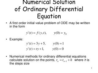
Numerical Solution of the Diffusivity Equation. Home. HOME. Introduction. Taylor Series Approximations. Numerical Approximation. Time Expansion. Explicit Difference Equation. Discrete Systems. Programming Exercise. Resources. Learning Objectives. Learning objectives in this module

E N D
Home HOME Introduction Taylor Series Approximations Numerical Approximation Time Expansion Explicit Difference Equation Discrete Systems Programming Exercise Resources
Learning Objectives • Learning objectives in this module • Develop problem solution skills using computers and numerical methods • Review the Gaussian elimination method for solving simultaneous linear equations • Develop programming skills using FORTRAN • FORTRAN elements in this module • -input/output • -do-loops • -subroutines • -common blocks
Introduction x=L Qin x=0 • The figure below shows a horizontal porous rod, where fluid is being injected into the left face at a flow rate Q. The injected fluid will be transported through the rod and eventually be produced out of the right face of the rod. • The partial differential equation (PDE) for this system, in it’s simplest form, is called the linear diffusivity equation. It is valid for one-dimensional flow of a liquid in a horizontal system, where it is assumed that porosity (f), viscosity (m), permeability (k) and compressibility (c) all are constants. It may be written as: • (1) PR Continue PL Qout
Introduction • This simplified equation may be solved analytically. For instance, if the initial pressure of the rod is PR, and we assume constant pressures at the end faces, PL and PR for left and right faces, respectively, we have the following analytical solution: • (2) • The pressure solution is dependent on position, x, as well as time, t. As time increases, the exponential term becomes smaller, and eventually the solution reduces to the steady-state form: • (3) Continue Continue
Introduction • The derivation of the analytical solution of the diffusivity equation is the same as was used in the previous module. • For real systems involving fluid flow in reservoirs, however, we are seldom able to obtain analytical solutions to the flow equations. This is because the reservoir properties are not constant, and the reservoir geometry is normally very complex. Therefore, most of the time we need to solve the equations numerically. In the next section, we will give a brief introduction to discrete systems and finite difference solutions. Gas Oil Water Remember that it doesn’t always look like this...
Discrete Systems • In order to solve Eq. (1) numerically by means of the finite difference method, we need to go from a continuous system description, as shown in Fig. 1, to a discrete system. To discretize, we simply divide the porous rod into a number of grid blocks, as shown below: • A system of N grid blocks, each of length x, now defines the discrete system. This type of grid is called a block-centered grid, and the grid blocks are assigned indices, i, referring to the mid-point of each block, representing the average property of the block. i+1 1 i N i-2 i-1 i+2 Click in each block to see its index x
Taylor Series Approximations • Next, we need to convert Eq. (1) from a continuous partial differential form to a discrete difference form. For this, we make use of the well-known Taylor series expansions. A function may be expressed in terms of and its derivatives as: • (4) • Replacing the function f(x) with pressure P(x,t), we may write the following expansions along the x-axis (at constant time, t ): • Forwards • Backwards Continue (5) (6)
Taylor Series Approximations • By adding the two expressions, and solving for the second derivative, we get the following expression: • By neglecting the higher order terms, we may write the following approximation • This is called a central approximation of the second derivative. The smaller the grid blocks used, the smaller will be the error involved. • For simplicity, we will change the notation, so that the grid index system is used for indicating position (grid block), and a superscript is used to indicate time level: (7) (8) Continue (9)
Time Expansion • At constant position, x, the pressure function may be expanded in forward direction with regard to time: • By solving for the first derivative, and neglecting the higher order terms, we obtain the following approximation: • or, by employing the index system: (9) (10) (11)
Explicit Difference Equation • Now, we may substitute Eqs. (9) and (11) into Eq. (1), and obtain the difference equation needed for the numerical solution: • Actually, Eq. (12) is not valid for the end blocks, ie. blocks 1 and N. These blocks need some special treatment because the blocks i-1 and N+1 that enter into the formulas do not exist. We will not get into the derivations for these blocks here, but give the results below. The complete form of Eq. (12) becomes: (12) Continue (13)
Explicit Difference Equation • The initial conditions and the boundary conditions are: • In the numerical solution procedure, the two boundary conditions are applied immediately, so that they in practice also are initial pressures
Explicit Difference Equation • We may now solve Eq. (13) for average pressures in grid blocks (i=1,...,N) explicitly. The solution starts at time t= t, and we solve for all pressures at that time level, since all pressures at t=0 are known. Then we proceed to the next time step, and solve for pressures at t=2P, since all pressures at t=t now are known, and so on. In the computer program, we will let index I represent the grid block position, and index J represent time level. Thus, we have the following system of equations to be programmed: • Here, Jmax is the total number of time steps Continue (15)
Program Exercise • This programming exercise involves the construction of a reservoir simulation program, although in a very simple form. The following steps should be carried out: • Make a FORTRAN program that solves the set of equations given in Eq. (15), and writes the computed pressures in each grid block to an ouput file, for each time step (t=0, t, 2 t, 3 t,...) . The FORTRAN program should also include the analytical solution (exercise 8), and the results should be written to the output file together with the numerical solution. • Organize the program so that you have a main program for input and output, and that calls a subroutine ANALYTICAL for analytical solution, and another subroutine FINITEDIFF for the numerical solution.
Program Exercise • Run the program with the following data: • N=10 k=1,0 Darcy P0=1 atm • L=100 cm =1,0 cP PR=1 atm • A=10 cm3 c=0,0001 atm-1 PL=2 atm • t=0,0005 s =0,2 • Run the program for 600 time steps, so that the pressures are beginning to stabilize. Write only the results to file every 10th step. • Use Excel or another plotting program to plot pressures in grid block number 1 (x=5 cm) vs. time, both for numerical and analytical solutions, so that you can get an impression of the numerical error involved in the numerical solution.
Resources Introduction to Fortran Fortran Template here The whole exercise in a printable format here Web sites • Numerical Recipes In Fortran • Fortran Tutorial • Professional Programmer's Guide to Fortran77 • Programming in Fortran77
General information About the author
FAQ • No questions have been posted yet. However, when questions are asked they will be posted here. • Remember, if something is unclear to you, it is a good chance that there are more people that have the same question For more general questions and definitions try these Dataleksikon Webopedia Schlumberger Oilfield Glossary
References W. H. Preuss, et al., “Numerical Recipes in Fortran”, 2nd edition Cambridge University Press, 1992 • References to the textbook : Chapter 19 - Partial Differential Equations • The Textbook can also be accessed online: Numerical Recipes in Fortran
Summary Subsequent to this module you should... • be able to effectively use Fortran • know the different program structures, such as Nag routines and subroutines • know the format constructions