Download
1 / 117
1.18k likes | 1.51k Views
Capital Structure Basics. Chapter 13. Learning Objectives. Break-even level of sales. Operating and financial leverage and risk. Risks and returns of leveraged buy-outs (LBOs). Effect of capital structure on value. Break-even Analysis. Steps to Solution

E N D
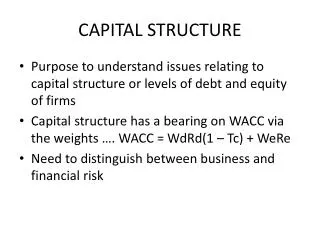
Capital Structure Basics Chapter 13
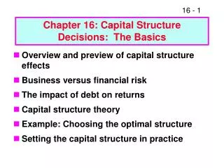
Learning Objectives • Break-even level of sales. • Operating and financial leverage and risk. • Risks and returns of leveraged buy-outs (LBOs). • Effect of capital structure on value.
Break-even Analysis • Steps to Solution • Construct a chart to find the sales break-even point = level of sales necessary to cover operating (not financial) costs. • This requires that you calculate EBIT for different unit sales amounts. • The point at which EBIT = 0 is the break-even level of sales.
Costs $ Units Produced Break-even Analysis • Assumptions • Fixed costs remain constant as quantity changes. • Variable costs vary as quantity of output changes. Variable Costs Fixed Costs
Fixed vs. Variable Costs • Fixed costs may include salaries, depreciation, rent. • Variable costs may include commissions, materials, labor. • This is a generalization. For example, some salaries may be considered fixed and others variable. In the long-run all costs are variable.
EBIT = Sales – Variable Costs - Fixed Costs Break-even Analysis • Calculation of Break-even Quantity Find Quantity which results in EBIT = $0
FC p – vc Unit Salesbe = Break-even Analysis • Calculation of Break-even Quantity Where: Unit Salesbe = Break-even quantity FC = Total fixed costs p = Sales price per unit vc = Variable costs per unit
FC p – vc Unit Salesbe = Break-even Analysis • Calculation of Break-even Quantity Example: Fixed Costs = $1,000,000/year Price = $800/unit Variable Costs = $400/unit
FC p – vc Unit Salesbe = $1,000,000 $800 – $400 = = 2,500 units Break-even Analysis • Calculation of Break-even Quantity Example: Fixed Costs = $1,000,000/year Price = $800/unit Variable Costs = $400/unit
TR = p x Q Break-even Analysis • Now calculate total revenue. p = Sales price per unit Q = unit sales
TR = p x Q Break-even Analysis • Calculate total revenue for different levels of sales. Unit sales (Q) xPrice (p)= Total Revenue (TR) 0 x $800 = $ 0 500 x $800 = $ 400,000 1,000 x $800 = $ 800,000 2,000 x $800 = $1,600,000 2,500 x $800 = $2,000,000
The Concept of Leverage You cannot easily move a large boulder.
The Concept of Leverage However, with the aid of a lever you can move an object many times your size.
The Concept of Leverage The longer the lever, the bigger the rock you can move.
The Concept of Leverage • In a financial context, the magnifying power of leverage can be used to help (or hurt) a firm’s financial performance. • Operating leverage occurs due to fixed costs in the production process. • With high fixed operating costs, a small change in sales will trigger a large change in operating income (EBIT).
% Change in EBIT % Change in Sales DOL= Operating Leverage • Measurement of Operating Leverage • Degree of Operating Leverage (DOL) • DOL > 1 means the firm has operating leverage.
% Change in EBIT % Change in Sales DOL= 100 33.33 ($1 - $.5) / $.5 ($4 - $3) / $3 DOL= = = 3.0 Operating Leverage • Example:S1 = 3,750 units S2 = 5,000 units • FC = $1mil and VC = $400/unit P = $800/unit • Sales of 3,750 units = (3,750 * $800) = $3mil • EBIT = $3mil - $1mil – $1.5mil= $.5mil • Sales of 5,000 units = (5,000 * $800) = $4mil • EBIT = $4mil - $1mil - $2mil = $1mil
Sales - Total VC Sales -Total VC - FC DOL= Operating Leverage • Measurement of DOL • Calculation using alternate formula:
Sales - Total VC Sales -Total VC - FC DOL= Operating Leverage • Measurement of DOL • Calculation using alternate formula: DOL = ($3 - $1.5) / ($3 - $1.5 - $1) = 1.5 / .5 = 3
Sales - Total VC Sales -Total VC - FC DOL= Q = 3,750 units P = $800 per unit VC = $400 per unit FC = $1,000,000 per year. Example: Operating Leverage • Measurement of DOL • Calculation using per unit information:
Sales - Total VC Sales -Total VC - FC DOL= 3,750(800) – 3,750(400) 3,750(800) –3,750(400) – 1,000,000 DOL3,750 units = Operating Leverage • Measurement of DOL • Calculation using per unit information: Interpretation: If sales change 1%, then EBIT will change 3% (same direction). = 3
Quantity DOL 2,500 (Qbe) Undefined 3,250 4.33 3,750 3 5,000 2 Operating Leverage • Degree of Operating Leverage falls as sales rise
Quantity DOL 2,500 (Qbe) Undefined 3,250 4.33 3,750 3 5,000 2 Operating Leverage • Degree of Operating Leverage falls as sales rise • The higher the sales level above break-even, the less the percent change in EBIT for a given percent change in sales • If FC = $0, DOL = 1
Leverage Table Number 1
% Change in NI % Change in EBIT DFLEBIT = Financial Leverage • Degree of Financial Leverage • Finance a portion of the firm’s assets with securities that have fixed financial costs • Debt • Preferred Stock • Financial Leverage measures changes in earnings per share as EBIT changes. Base Level of EBIT
% Change in NI % Change in EBIT DFL= 167 100 (480.6 - 180) / 180 ($1 - $.5) / $.5 DFL= = = 1.67 Financial Leverage Example: EBIT1 = $500,000 EBIT2 = $1,000,000 NI1 = $180,000 NI2 = $480,600
EBIT EBIT – I DFLEBIT = Financial Leverage • Measurement of DFL (Alternate formula) • If DFL > 1, the firm has financial leverage. A given percent change in EBIT will result in a larger percent change in NI.
500,000 500,000 – 200,000 DFLEBIT=500,000 = Financial Leverage Example: EBIT = $500,000 Interest Charges = $200,000 = 1.67 times Interpretation: When EBIT changes 1% (from an existing level of $50,000) Net Income will change 1.67% in the same direction.
Leverage Table Number 1
% Change in NI % Change in Sales DCLS = Combined Leverage • Degree of Combined Leverage • Measures changes in Net Income given changes in Sales • Combines both Operating and Financial Leverage • Computed for a specific level of sales Base Level of Sales
% Change in NI % Change in Sales DCL= 166.7 33.3 (480.6 - 180) / .180 ($4 - $3) / $3 DCL= = = 5.0 Combined Leverage Example: SALES1 = $3,000,000 SALES2 = $4,000,000 NI1 = $180,000 NI2 = $480,600
DCLS = DOLS x DFLEBIT Example: DOLS = 3.0 DFLEBIT = 1.67 Combined Leverage DCL3,750 = 3.0x 1.67 = 5.0 times
Sales – VC Sales - VC - FC - I DCLS = 3,750(800) – 3,750(400) 3,750(800) – 3,750(400) – 1,000,000 - $200,000 DCL3,750 = 3 mil – 1.5 mil 3 mil – 1.5 mil – 1 mil - .2 mil = Combined Leverage Example: = 1,500,000 300,000 = 5
DCLS = DOLS x DFLEBIT DCLS = DOLS x DFLEBIT Example: DOLS = 3.0 DFLEBIT = 1.67 Combined Leverage DCL3,750 = 3.0x 1.67 = 5.0 times Interpretation: When sales change 1%, Net Income will change 5.0% in the same direction
Leverage Table Number 1
Effect of Leverage • Leverage can help the firm or hurt it. • If EBIT increases, financial leverage will magnify the increase in net income. • If EBIT decreases, financial leverage will magnify the decrease in net income.
Capital Structure Theory • Capital Structure is the mixture of sources of funds a firm uses. • Debt • Preferred Stock • Common Stock
Capital Structure Theory • A benefit of debt financing is that interest is tax deductible to the paying firm whereas payments to equity providers are not. • Firms must trade-off this benefit against the increased financial risk associated with higher debt levels.
Capital Structure TheoryModigliani and Miller (M&M) • M&M wrote an important paper in 1958 in which they proved that with certain assumptions there is no optimal capital structure. One is as good as any other. • M&M’s Assumptions: No transaction costs, no taxes, everyone has same information and borrowing rates, debt is riskless, debt does not affect operations.
Capital Structure TheoryModigliani and Miller (M&M) • In a later paper, M&M showed that when the tax deductibility of interest is considered, their model indicates that a capital structure of 100% debt is optimal.
Capital Structure in the Real World • Firms attempt to balance the costs and benefits of debt to reach the optimal mix that maximizes the value of the firm. • Affect on costs of capital: • Since debt is cheaper than equity, use of debt will initially lower the WACC. • At high levels of debt, the WACC will increase as investors perceive the risk of the firm to be increasing substantially.
Cost of Capital and Capital Structure kd ks ks ka ka K* kd We minimize K* at 50% debt
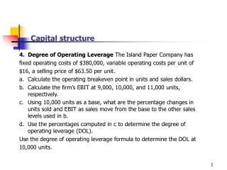
Homework Problems 1. You are given the following information for Firm XYZ: Fixed operating costs = $500,000 Variable operating costs per unit = $40/unit Sales price per unit = $50/unit Calculate the break-even point in units for: (treat each scenario independently) a. fixed costs decrease to $450,000 b. variable cost decreases to $37 per unit c. sales price increases to $55/unit d. changes for a, b, c, occur simultaneously 2. Company X has a sales price of $4.00 per unit and a variable cost of $3.40 per unit; fixed costs are $13,000, no debt, and sales of 250,000 units per year. Company Y has a sales price of $10.00 per unit and a variable cost of $7.00 per unit with fixed costs of $135,000 and sales of 200,000 units per year. Company Y also has interest payments of $60,000 annually. Both companies are in the 40% tax bracket. a. compute DOL, DFL, and DCL for Company X b. compute DOL, DFL, and DCL for Company Y c. compare the relative risk of both companies 3. Why is the Modigliani and Miller theory of capital structure not really practical for firms in the real world? 4. Debt financing is often called a two-edged sword. What does this mean? 5. Given a net income of $50,000, sales of $2,000,000, variable costs of $25,000, fixed operating costs of $175,000, price per unit of $5.00, interest expense of $20,000, and EBIT of $1,800,000: a. calculate DOL b. calculate DFL c. calculate DCL
Corporate Bonds, Preferred Stock, and Leasing Chapter 14
Learning Objectives • Bond contract terms • Differences among types of bonds • Features of preferred stock • Lease versus purchase • Balance sheet treatment of leases
Bond Basics • Bondholders are lending the corporation funds for some stated period of time. • The corporation promises to make certain payments to the owner of the bond.
Bond Basics • Indenture • Definition: the contract between the corporation and the investor • Provisions included in the indenture: • par value • coupon rate and payment dates • maturity date • any special features
Bond Basics • Par Value • (e.g. $1,000) also called Face Value • Coupon Interest Rate • The stated rate of interest. The rate that is multiplied by the par value to determine the annual dollar interest paid. • Maturity • Time at which the original principal (Par Value) is repaid to the bondholder.
Special Features of Bond Indentures • Collateral • If the debt is secured by specific assets, the lender is entitled to take the assets in the event of default. • Plan for repayment at maturity • Staggered maturities makes it easier for the firm to raise the necessary funds. Sinking funds allow the firm to set aside the funds over time to ensure the ability to repay the loan.
Special Features of Bond Indentures • Provisions for early repayment • Call provisions allow the issuer to refinance the debt, usually done if interest rates fall. • Issuing new bonds to replace old bonds is known as refunding.