Download
1 / 19
190 likes | 427 Views
The Backward Error Compensation Method for Level Set Equation. Wayne Lawton and Jia Shuo Email: matwml@nus.edu.sg Department of Mathematics National University of Singapore. Level Set Method (Osher and Sethian 1988).

E N D
The Backward Error Compensation Method for Level Set Equation Wayne Lawton and Jia Shuo Email: matwml@nus.edu.sg Department of Mathematics National University of Singapore
Level Set Method (Osher and Sethian 1988) • The interface is represented as a zero level set of a Lipschitz continuous function φ(x,t) • The evolution equation of φ(x,t) under a velocity field u: Φt + u · grad φ= 0
Applications • Multiphase flows • Stefan problem • Kinetic crystal growth • Image processing and computer vision • Advantages • Naturally handle topological changes and complex geometries of the interfaces • Simple formulae for unit normal and curvature n = gradφκ= div (gradφ/|gradφ|)
Conventional Numerical Schemes • Schemes for hyperbolic conservation laws • Spatial: Essential Non-Oscillatory (ENO) • Temporal: Total Variation Diminishing Runge-Kutta (TVD-RK)
Backward Error Compensation (Dupont and Liu 2003) Consider the ODE: y’= f(t,y) • Advance it one step from tn to tn+1 by forward Euler method: y1n+1= yn + Δt fn • Solve the ODE backward from tn+1 to tn y2n = y1n+1 - Δt fn+1 • If no numerical errors, yn = y2n. Let e = yn - y2n
Assume that the errors in the forward and backward process are the same. Let y3n = yn + e/2 = yn + (yn - y2n)/2 • Starting with y3n to remove the principal components of the error at tn+1, solve the ODE forward again. yn+1 = y3n + Δt f(tn,y3n)
Backward Error Compensation yn+1 = yn + Δt(fn+1 + f(tn,y3n) – fn)/2 • 2nd order modified Euler scheme yn+1 = yn + Δt(fn+1 + fn)/2 • (fn+1 + f(tn,y3n) – fn) - (fn+1 + fn) =O(Δt2) The forward Euler with backward error compensation is 2nd order accuracy
Theorem: The backward error compensation algorithm can improve the order of accuracy of kth order Taylor method yn+1= yn + Δt fn + Δt2f’n/2 + …+ Δtk f(k-1)n /k! by one if k is an odd positive number.
Consider 1-D level set equation Φt + uφx = 0 • 1st order upwind scheme for φx (φx)i = (φi – φi-1 )/Δx, if ui > 0 (φi+1 – φi )/Δx, if ui < 0 • Assume u =1, the 1st order upwind scheme can be written as Φn+1i = (1-λ) φni + λφni-1, where λ= Δt/Δx.
Applying the backward error compensation, Φn+1i = (λ2/2+λ3/2) φni-2 + (λ/2+2 λ2-3λ3)φni-1 + (1-5λ2/2+3λ3/2)φni + (-λ/2+λ2-λ3 /2)φni+1 (1) • The local truncation error is O(Δx3) • It not only improves the temporal order of accuracy by one, but also improves the spatial order by one.
Stable Condition • Theorem: If 0<λ ≤1.5 and un+1 is defined by (1) with periodic boundary condition, then ||un+1||2≤ ||un||2. Proof: by expansion in Fourier series. Remark: Backward error compensation with center difference creates a stable scheme for 0<λ ≤31/2.
Reinitialization • Keep Φ as a distance function at each time step • PDE approach Φτ= sgn(Φ0)(1-|gradΦ|) Φ(x,0) = Φ0(x) • ENO and TVD-RK
For the grid x near the interface, we do a Taylor expansion to find an accurate approximation of the orthogonal projection y of x on the interface. • y = x + rp, where p = grad φ/|grad φ| • Φ(x) + |grad φ |r + (pTH(φ)p) r2 = φ(y) = 0, where H is the Hessian matrix of φ. • Then r is the distance from x to the interface. y p x
Accuracy Check Move a unit circle Φ0=(x2 + y2)1/2-1 with a constant velocity (1,1) in a 4x4 periodic box.
Numerical Results • Rotational Velocity Field Rotate a slotted disk in a 100x100 square with the velocity field u(x,y) = pi(50-y)/314; v(x,y) = pi(x-50)/314. We compute for t=628 on a 200x200 grid.
T = 0 T = 628
Applications in Multiphase Flows • Solve Navier-Stokes equation using projection method • Solve the level set equation using backward error compensation • Reinitialization by solving the quadratic equation near the interface
Numerical Examples ρw/ ρA = 100; μw/ μA = 10 Δx=Δy=0.005; Δt=0.001