Projects

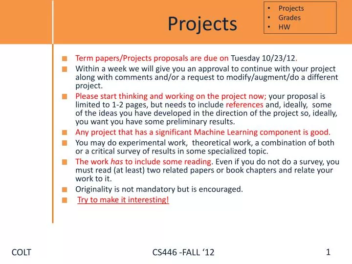
1. Projects • Projects • Grades • HW • Term papers/Projects proposals are due on Tuesday 10/23/12. • Within a week we will give you an approval to continue with your project along with comments and/or a request to modify/augment/do a different project. • Please start thinking and working on the project now; your proposal is limited to 1-2 pages, but needs to include references and, ideally, some of the ideas you have developed in the direction of the project so, ideally, you want you have some preliminary results. • Any project that has a significant Machine Learning component is good. • You may do experimental work,  theoretical work, a combination of both or a critical survey of results in some specialized topic. • The work has to include some reading. Even if you do not do a survey, you must read (at least) two related papers or book chapters and relate your work to it. • Originality is not mandatory but is encouraged. • Try to make it interesting!

2. Examples • Health Application: Learn access control rules to medical records • Work on making learned hypothesis (e.g., linear threshold functions) more comprehensible (medical domain example) • Develop a People Identifier • Compare Regularization methods: e.g., Winnow vs. L1 Regularization • Deep Networks: convert a state of the art NLP program to a deep network, efficient, architecture. • Try to prove something • Try to make it interesting! • PDF 2 Text • Convert PDF files to text – focus on tables, captions,… • Conference Program Chair Aid • Identify if the paper is anonymous • Twitter • Identify Gender • Identify Age • Parse #hashtags: • #dontwantmygradprogramfollowingme • #Rothhashana • Conference Program Chair Aid • Author identification (especially difficult for multi-authored papers)

3. Where are we? • Algorithmically: • Perceptron + Winnow • Gradient Descent • Models: • Online Learning; Mistake Driven Learning • What do we know about Generalization? (to previously unseen examples?) • How will your algorithm do on the next example? • Next we develop a theory of Generalization. • We will come back to the same (or very similar) algorithms and show how the new theory sheds light on appropriate modifications of them, and provides guarantees.

4. Computational Learning Theory • What general laws constrain inductive learning ? • What learning problems can be solved ? • When can we trust the output of a learning algorithm ? • We seek theory to relate • Probability of successful Learning • Number of training examples • Complexity of hypothesis space • Accuracy to which target concept is approximated • Manner in which training examples are presented

5. Quantifying Performance • We want to be able to say something rigorous about the performance of our learning algorithm. • We will concentrate on discussing the number of examples one needs to see before we can say that our learned hypothesis is good.

6. Learning Conjunctions • There is a hidden conjunction the learner (you) is to learn • How many examples are needed to learn it ? How ? • Protocol I: The learner proposes instances as queries to the teacher • Protocol II: The teacher (who knows f) provides training examples • Protocol III: Some random source (e.g., Nature) provides training examples; the Teacher (Nature) provides the labels (f(x))

7. Learning Conjunctions • Protocol I: The learner proposes instances as queries to the teacher • Since we know we are after a monotone conjunction: • Is x100 in? <(1,1,1…,1,0), ?> f(x)=0 (conclusion: Yes) • Is x99 in? <(1,1,…1,0,1), ?> f(x)=1 (conclusion: No) • Is x1 in ? <(0,1,…1,1,1), ?> f(x)=1 (conclusion: No) • A straight forward algorithm requires n=100 queries, and will produce as a result the hidden conjunction (exactly). What happens here if the conjunction is not known to be monotone? If we know of a positive example, the same algorithm works.

8. Learning Conjunctions • Protocol II: The teacher (who knows f) provides training examples • <(0,1,1,1,1,0,…,0,1), 1> (We learned a superset of the good variables) • To show you that all these variables are required… • <(0,0,1,1,1,0,…,0,1), 0> need x2 • <(0,1,0,1,1,0,…,0,1), 0> need x3 • ….. • <(0,1,1,1,1,0,…,0,0), 0> need x100 • A straight forward algorithm requires k = 6 examples to produce the hidden conjunction (exactly). Modeling Teaching Is tricky

9. Learning Conjunctions • Protocol III: Some random source (e.g., Nature) provides training examples • Teacher (Nature) provides the labels (f(x)) • <(1,1,1,1,1,1,…,1,1), 1> • <(1,1,1,0,0,0,…,0,0), 0> • <(1,1,1,1,1,0,...0,1,1), 1> • <(1,0,1,1,1,0,...0,1,1), 0> • <(1,1,1,1,1,0,...0,0,1), 1> • <(1,0,1,0,0,0,...0,1,1), 0> • <(1,1,1,1,1,1,…,0,1), 1> • <(0,1,0,1,0,0,...0,1,1), 0>

10. Learning Conjunctions • Protocol III: Some random source (e.g., Nature) provides training examples • Teacher (Nature) provides the labels (f(x)) • Algorithm: Elimination • Start with the set of all literals as candidates • Eliminate a literal that is not active (0) in a positive example • <(1,1,1,1,1,1,…,1,1), 1> • <(1,1,1,0,0,0,…,0,0), 0> learned nothing • <(1,1,1,1,1,0,...0,1,1), 1> • <(1,0,1,1,0,0,...0,0,1), 0> learned nothing • <(1,1,1,1,1,0,...0,0,1), 1> • <(1,0,1,0,0,0,...0,1,1), 0> Final hypothesis: • <(1,1,1,1,1,1,…,0,1), 1> • <(0,1,0,1,0,0,...0,1,1), 0> We can determine the # of mistakes we’ll make before reaching the exact target function, but not how many examples are need to guarantee good performance. Is that good ? Performance ? # of examples ?

11. Two Directions • Can continue to analyze the probabilistic intuition: • Never saw x1 in positive examples, maybe we’ll never see it? • And if we will, it will be with small probability, so the concepts we learn may be pretty good • Good: in terms of performance on future data • PAC framework • Mistake Driven Learning algorithms • Update your hypothesis only when you make mistakes • Good: in terms of how many mistakes you make before you stop, happy with your hypothesis. • Note: not all on-line algorithms are mistake driven, so performance measure could be different. Two Directions

12. Prototypical Concept Learning • Instance Space: X • (animals; described by attributes, such as Barks (Y/N), has_4_legs (Y/N),…) • Concept Space: C • set of possible target concepts (dog=(barks=Y) (has_4_legs=Y)) • Hypothesis Space:H set of possible hypotheses • Training instances S: positive and negative examples of the target concept f  C • Determine: A hypothesis h  H such that h(x) = f(x) • A hypothesis h  H such that h(x) = f(x) for all x  S ? • A hypothesis h  H such that h(x) = f(x) for all x  X ?

13. Prototypical Concept Learning • Instance Space: X • (animals; described by attributes, such as Barks (Y/N), has_4_legs (Y/N),…) • Concept Space: C • set of possible target concepts (dog=(barks=Y) (has_4_legs=Y)) • Hypothesis Space:H set of possible hypotheses • Training instances S: positive and negative examples of the target concept f  C training instances are generated by a fixed unknown probability distribution D over X • Determine: A hypothesis h  H that estimates f, evaluated by its performance on subsequent instances x  Xdrawn according toD

14. PAC Learning – Intuition • We have seen many examples (drawn according to D ) • Since in all the positive examplesx1was active, it is very likely that it will be • active in future positive examples • If not, in any case, x1 is active only in a small percentage of the • examples so our error will be small - f h + + - - f and h disagree

15. The notion of error • Can we bound the Error • given what we know about the training instances ? - f h + + - - f and h disagree

16. - f h + + - - Learning Conjunctions– Analysis (1) • Let z be a literal. Let p(z) be the probability that zis false in positive example sampled from D. Then: • p(z) is also the probability that z is deleted from h in a randomly chosen positive example. • If z is in the target concept, than p(z) = 0. • Claim: h will make mistakes only on positive examples. • A mistake is made only if a literal z, that is in hbut not in f is false in a • positive example. In this case, hwill say NEG, but the example is POS. • Thus, p(z) is also the probability that z causes h to make a mistake on a randomly drawn example from D . • There may be overlapping reasons for mistakes, but the sum clearly bounds it.

17. Learning Conjunctions– Analysis (2) • Call a literal z bad if p(z) > /n. • A bad literal is a literal that has a significant probability to appear with a positive example but, nevertheless, it has not appeared with one in the training data. • Claim: If there are no bad literals, than error(h) < . Reason: • What if there are bad literals ? • Let z be a bad literal. • What is the probability that it will not be eliminated by a given example? Pr(z survives one example) = 1- Pr(z is eliminated by one example) = = 1 – p(z) < 1- /n • The probability that z will not be eliminated by mexamples is therefore: Pr(z survives m independent examples) = (1 –p(z))m < (1- /n)m • There are at most n bad literals, so the probability that some bad literalsurvives m examples is bounded by n(1- /n)m

18. Learning Conjunctions– Analysis (3) • We want this probability to be small. Say, we want to choose m large enough such that the probability thatsome z survives m examples is less than . • (I.e., that z remains in h, and makes it different from the target function) Pr(z survives m example) = n(1- /n)m <  • Using 1-x < e-xit is sufficient to require that n e-m/n <  • Therefore, we need examples to guarantee a probability of failure(error > ²) of less than . • With =0.1, =0.1, and n=100, we need 6907 examples. • With =0.1, =0.1, and n=10, we need only 460 example, only 690 for =0.01

19. Formulating Prediction Theory • Instance Space X, Input to the Classifier; Output Space Y = {-1, +1} • Making predictions with: h: X  Y • D: An unknown distribution over X £ Y • S: A set of examples drawn independently from D; m = |S|, size of sample. Now we can define: • True Error: ErrorD = Pr(x,y) 2 D [h(x) : = y] • Empirical Error: ErrorS= Pr(x,y) 2 S [h(x) : = y] = 1,m [h(xi) := yi] • (Empirical Error (Observed Error, or Test/Train error, depending on S)) This will allow us to ask: (1)Can we describe/bound ErrorDgiven ErrorS? • Function Space: C – Aset of possible target concepts; target is: f: X  Y • Hypothesis Space:H – A set of possible hypotheses • This will allow us to ask: (2) Is C learnable? • Is it possible to learn a given function in C using functions in H, given the supervised protocol?

20. Requirements of Learning • Cannot expect a learner to learn a concept exactly, since • - there will generally be multiple concepts consistent with the available data • (which represent a small fraction of the available instance space). • - Unseen examples could potentially have any label (??) • - We “agree” to misclassify uncommon examples that do not show up in the • training set. • Cannot always expect to learn a close approximation to the target concept • since sometimes (only in rare learning situations, we hope) the training set • will not be representative. (will contain uncommon examples) • Therefore, the only realistic expectation of a good learner is that with high • probability it will learn a close approximation to the target concept.

21. Requirements of Learning • Cannot expect a learner to learn a concept exactly. • Cannot always expect to learn a close approximation to the target concept • since sometimes (only in rare learning situations, we hope) the training set • will not be representative. (will contain uncommon examples) • Therefore, the only realistic expectation of a good learner is that with high • probability it will learn a close approximation to the target concept. • In Probably Approximately Correct (PAC) learning, one requires that • given small parameters  and , with probability at least (1- ) • a learner produces a hypothesis with error at most  • The reason we can hope for that is theConsistent Distribution assumption.

22. PAC Learnability • Consider a concept class C • defined over an instance space X (containing instances of length n), • and a learner L using a hypothesis space H. • C is PAC learnable by L using H if • for all f  C, • for all distribution D over X, and fixed 0< ,  < 1, • L, given a collection of m examples sampled independently according to • the distributionD produces • with probability at least(1- ) a hypothesis h  H witherror at most  • (ErrorD = PrD[f(x) : = h(x)]) • where m is polynomial in 1/ , 1/ , n and size(C) • C is efficiently learnable if L can produce the hypothesis • in time polynomial in 1/ , 1/ , n and size(C)

23. PAC Learnability • We impose two limitations: • Polynomial sample complexity (information theoretic constraint) • Is there enough information in the sample to • distinguish a hypothesis h that approximate f ? • Polynomial time complexity (computational complexity) • Is there an efficient algorithm that can process the sample • and produce a good hypothesis h ? • To be PAC learnable, there must be a hypothesis h  H with arbitrary small error • for every f C. We generally assume H  C. (Properly PAC learnable if H=C) • Worst Case definition: the algorithm must meet its accuracy • for every distribution (The distribution free assumption) • for every target function f in the class C

24. Proof: Let h be such a bad hypothesis. - The probability that h is consistent with one example of f is - Since the m examples are drawn independently of each other, The probability that h is consistent with m example of f is less than - The probability that some hypothesis in H is consistent with m examples is less than Occam’s Razor (1) Claim: The probability that there exists a hypothesis h  Hthat (1) is consistent with m examples and (2) satisfies error(h) > ( ErrorD(h) = Prx 2 D [f(x) :=h(x)] ) is less than |H|(1-  )m . Note that we don’t need a true f for this argument; it can be done with h, relative to a distribution over X £ Y.

25. Occam’s Razor (1) We want this probability to be smaller than , that is: |H|(1-) <  ln(|H|) + m ln(1-) < ln() (with e-x = 1-x+x2/2+…; e-x > 1-x; ln (1- ) < - ; gives a safer ) (gross over estimate) It is called Occam’s razor, because it indicates a preference towards small hypothesis spaces What kind of hypothesis spaces do we want ? Large ? Small ? To guarantee consistency we need H  C. But do we want the smallest H possible ? m What do we know now about the Consistent Learner scheme?

26. Consistent Learners • Immediately from the definition, we get the following general scheme for learning: • Given a sample D of m examples • Find some h  H that is consistent with all m examples • Show that if m is large enough, • a consistent hypothesis must be close enough to f • Show that you can compute the consistent hypothesis efficiently • In the case of conjunctions -- • We used the Elimination algorithm to find a hypothesis h that • is consistent with the training set (easy to compute) • We showed that if we have sufficiently many examples (polynomial • in the parameters), than h is close to the target function.

27. Examples n • Conjunction (general): The size of the hypothesis space is 3 • Since there are 3 choices for each feature • (not appear, appear positively or appear negatively) • (slightly different than previous bound) • If we want to guarantee a 95% chance of learning a hypothesis of at least 90% accuracy, • with n=10 Boolean variable, m > (ln(1/0.05) +10ln(3))/0.1 =140. • If we go to n=100, this goes just to 1130, (linear with n) • but changing the confidence to 1% it goes just to 1145 (logarithmic with ) • These results hold for any consistent learner.

28. K-CNF • Occam Algorithm for f  k-CNF • Draw a sample D of size m • Find a hypothesis h that is consistent with all the examples in D • Determine sample complexity: • Due to the sample complexity result h is guaranteed to be a PAC hypothesis; but we need to learn a consistent hypothesis. How do we find the consistent hypothesis h ?

29. K-CNF How do we find the consistent hypothesis h ? • Define a new set of features (literals), one for each clause of size k • Use the algorithm for learning monotone conjunctions, • over the new set of literals Example: n=4, k=2; monotone k-CNF Original examples: (0000,l) (1010,l) (1110,l) (1111,l) New examples: (000000,l) (111101,l) (111111,l) (111111,l) Distribution?

30. More Examples Unbiased learning: Consider the hypothesis space of all Boolean functions on n features. There are different functions, and the bound is therefore exponential in n. k-CNF: Conjunctions of any number of clauses where each disjunctive clause has at most k literals. k-clause-CNF: Conjunctions of at most k disjunctive clauses. k-DNF: Disjunctions of any number of terms where each conjunctive term has at most k literals. k-term-DNF: Disjunctions of at most k conjunctive terms.

31. Sample Complexity • All these classes can be learned using a polynomial size sample. • We want to learn a 2-term-DNF; what should our hypothesis class be? • k-CNF: Conjunctions of any number of clauses where each disjunctive clause has at most k literals. • k-clause-CNF: Conjunctions of at most k disjunctive clauses. • k-DNF: Disjunctions of any number of terms where each conjunctive term has at most k literals. • k-term-DNF: Disjunctions of at most k conjunctive terms.

32. Computational Complexity • Even though from the sample complexity perspective things are good, they are not good from a computational complexity in this case. • Determining whether there is a 2-term DNF consistent with a set of training data is NP-Hard. Therefore the class of k-term-DNF is not efficiently (properly) PAC learnable due to computational complexity • But, we have seen an algorithm for learning k-CNF. • And, k-CNF is a superset of k-term-DNF • (That is, every k-term-DNF can be written as a k-CNF) What does it mean?

33. Computational Complexity • Determining whether there is a 2-term DNF consistent with a set of training data is NP-Hard • Therefore the class of k-term-DNF is not efficiently (properly) PAC learnable due to computational complexity • We have seen an algorithm for learning k-CNF. • And, k-CNF is a superset of k-term-DNF • (That is, every k-term-DNF can be written as a k-CNF) • Therefore, C=k-term-DNF can be learned as using H=k-CNF as the hypothesis Space • Importance of representation: • Concepts that cannot be learned using one representation can be learned using another (more expressive) representation. C H

34. Negative Results – Examples • Two types of nonlearnability results: • Complexity Theoretic • Showing that various concepts classes cannot be learned, based on well-accepted assumptions from computational complexity theory. • E.g. : C cannot be learned unless P=NP • Information Theoretic • The concept class is sufficiently rich that a polynomial number of examples may not be sufficient to distinguish a particular target concept. • Both type involve “representation dependent” arguments. • The proof shows that a given class cannot be learned by algorithms using hypotheses from the same class. (So?) • Usually proofs are for EXACT learning, but apply for the distribution free case.

35. Negative Results for Learning • Complexity Theoretic: • k-term DNF, for k>1 (k-clause CNF, k>1) • Neural Networks of fixed architecture (3 nodes; n inputs) • “read-once” Boolean formulas • Quantified conjunctive concepts • Information Theoretic: • DNF Formulas; CNF Formulas • Deterministic Finite Automata • Context Free Grammars

36. Agnostic Learning • Assume we are trying to learn a concept f using hypotheses in H, but f  H • In this case, our goal should be to find a hypothesis h  H, with a small training error: • We want a guarantee that a hypothesis with a small training error will have a good accuracy on unseen examples • Hoeffding bounds characterize the deviation between the true probability of some event and its observed frequency over m independent trials. • (p is the underlying probability of the binary variable (e.g., toss is Head) being 1)

37. Agnostic Learning • Therefore, the probability that an element in H will have training error which is off by more than  can be bounded as follows: • Doing the same union bound game as before, with =|H|exp{2m2} , • We get a generalization bound – a bound on how much will the true error deviate from the observed error. • For any distribution D generating training and test instance, with probability at least 1- over the choice of the training set of size m, (drawn IID), for all hH

38. Agnostic Learning • An agnostic learner which makes no commitment to whether f is in H and returns the hypothesis with least training error over at least the following number of examples can guarantee with probability at least (1-) that its training error is not off by more than  from the true error. Learnability depends on the log of the size of the hypothesis space

39. Learning Rectangles • Assume the target concept is an axis parallel rectangle Y X

40. CS446-Fall 10 Learning Rectangles • Assume the target concept is an axis parallel rectangle Y + + - X

41. Learning Rectangles • Assume the target concept is an axis parallel rectangle Y + + - X

42. Learning Rectangles • Assume the target concept is an axis parallel rectangle Y + + - + + X

43. Learning Rectangles • Assume the target concept is an axis parallel rectangle Y + + - + + X

44. Learning Rectangles • Assume the target concept is an axis parallel rectangle Y + + + + - + + + + + + X

45. Learning Rectangles • Assume the target concept is an axis parallel rectangle Y + + + + + - + + + + + + X

46. Learning Rectangles • Assume the target concept is an axis parallel rectangle • Will we be able to learn the target rectangle ? Y + + + + + - + + + + + + X

47. Learning Rectangles • Assume the target concept is an axis parallel rectangle • Will we be able to learn the target rectangle ? • Can we come close ? Y + + + + + - + + + + + + X

48. Infinite Hypothesis Space • The previous analysis was restricted to finite hypothesis spaces • Some infinite hypothesis spaces are more expressive than others • E.g., Rectangles, vs. 17- sides convex polygons vs. general convex polygons • Linear threshold function vs. a conjunction of LTUs • Need a measure of the expressiveness of an infinite hypothesis space other • than its size • The Vapnik-Chervonenkis dimension (VC dimension) provides such • a measure • Analogous to |H|, there are bounds for sample complexity using VC(H)

49. Shattering

50. Shattering