Download
1 / 23
230 likes | 322 Views
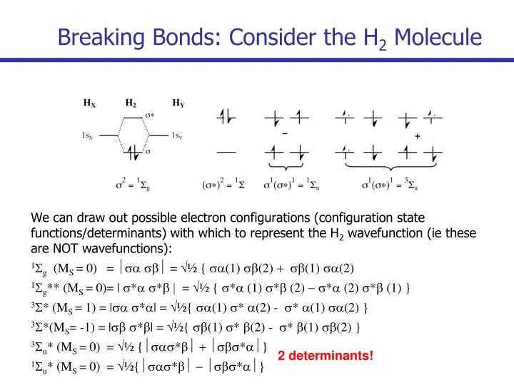
Breaking Bonds: Consider the H 2 Molecule. We can draw out possible electron configurations (configuration state functions/determinants) with which to represent the H 2 wavefunction ( ie these are NOT wavefunctions ):

E N D
Breaking Bonds: Consider the H2 Molecule We can draw out possible electron configurations (configuration state functions/determinants) with which to represent the H2wavefunction (ie these are NOT wavefunctions): 1Sg (MS = 0) = ½sa sb½ = ½ { sa(1) sb(2) + sb(1) sa(2) 1Sg** (MS = 0)= | s*a s*b | = ½{ s*a (1)s*b(2) -s*a (2)s*b(1) } 3S* (MS = 1) = |sas*a| = ½{ sa(1) s* a(2) - s* a(1) sa(2) } 3S*(MS= -1) = |sbs*b| = ½{ sb(1) s* b(2) - s* b(1) sb(2) } 3Su* (MS = 0) = ½ {½sas*b½ +½sbs*a½} 1Su* (MS = 0) = ½{½sas*b½ -½sbs*a½} 2 determinants!
H2 molecule • As the RHH bond stretches and breaks, the s and s* orbitals become degenerate, approaching the energy of a H 1s orbital
H2 molecule • Expand out the lowest energy determinant: 1Sg = ½sa sb½ = ½ ½ (sx + sy) a (sx + sy) b½ = ½ {½sxa sxb½+½sya syb½+½sxa syb½+½sya sxb½} = ½ { HX·· + HY + HX + HY·· + HX· + HY· + HX· + HY· } E(1Sg) ½ [E (HX·) + E (HX·) + E (HX) + E ( HX·· ) ] ie the average of the covalent energy { E (HX·) + E (HX·) } and the ionic energy { E (HX) + E ( HX·· ) } H- + H+ ionic H + H covalent H+ + H- ionic H + H covalent
H2 molecule • Get limits for other determinants as RHH∞ and plot the energy of the determinants as a function of RHH: 1Sg** E (HX··) + E (HY) ½ [ E (HX·) + E (HY·)+E (HX··) + E (HY) ] E (HX·) + E (HX·) 1Sg Described well as a single determinant
H2 molecule • Get limits for other determinants as RHH∞ and plot the energy of the determinants as a function of RHH: 1Sg** E (HX··) + E (HY) ½ [ E (HX·) + E (HY·)+E (HX··) + E (HY) ] E (HX·) + E (HX·) 1Sg Described well as a single determinant Determinants have the same symmetry and can interact
H2 molecule • Mix the determinants to get the wavefunctions – the combination of determinants will vary with RHH: 1Sg** E (HX··) + E (HY) E (HX·) + E (HX·) 1Sg Now we dissociate to the right things…
H2 molecule • At intermediate RHH distances, the 1Sg and 1Sg** valence determinants interact: multiconfigurationproblem • The triplet dissociation is well behaved... • singlet-triplet instability – the spin-paired wave function is unstable with respect to relaxation of the spin symmetry ie the energies of the individual singlet and triplet determinants cross • This instability occurs at a threshold when the exchange interaction between the electrons involved exceeds their orbital energy difference • That is, tesinglet-triplet instability arises from competition between spin-pairing in a bond and spin localization in separated atoms. • Somewhat unfortunately, the singlet-triplet instability is ubiquitous when studying breaking bonds and can be much worse for multiple bonds…
Excited States • Koopman’s Theorem: the molecular orbital energy approximates energy required to ionize an electron from that orbital. • Energies of the occupied andunoccupied (virtual) molecularorbitalscan be used to approx-imate excitation energies forexcitation between two orbitals • BUT energies ofvirtual orbitalsactually correspond to stateswith N electrons whereas electron in virtual orbital should only see N-1 electrons
Methods for Excited States • Ground State Methods • a ground state method can be used to calculate the lowest energy state for each possible spin multiplicity (2S+1) • a ground state method can be used to calculate the lowest energy state for each possible irreducible representation of the wavefunction in the molecular point group (spatial symmetry) • Single Reference Methods for Excited States • ONLY if the excited state is dominated by a single determinant or if the multi-configurational excited states (eg open shell singlets) are correctly described by single reference methods provided their wavefunctions are dominated by single-electron excitations • Closed shell species at equilibrium geometries • Some doublet radicals • Some triplet diradicals
Methods for Excited States • Configuration Interaction Single Excitations (CIS) • The CIS wavefunction starts with an optimized HF reference wavefunction • All the “excited” Slater determinants representing single electron excitations from the O occupied orbitalsto the V virtual (unoccupied) orbitalsare constructed and the electronic wavefunction is expanded as a linear combination of these determinants, ia, with coefficients in this expansion, cia , are determined variationally • Diagonalizing the matrix representation of the Hamiltonian in the space of singly excited determinants yields eigenvalues corresponding to the energies of the ground and excited states and eigenvectors corresponding to the ground and excited electronic state wavefunctions.
CIS: Properties and Limitations • Can be applied to larger molecules • The CIS wavefunction is variationalie excited state energies are upper bounds to the exact energies • The excited state wavefunctions are orthogonal to the ground state wavefunction • CIS is size consistent • It is possible to obtain pure singlet and pure triples states for closed shell molecules. • The CIS excited state wavefunctions are “well-defined” • The CIS energy is analytically differentiable efficient optimizations
CIS: Properties and Limitations • Does not explicitly include correlation through the ground state wavefunction • In general excitation energies at CIS are too large by 0.5-2 eV compared with experiment. • The “singly excited” HF determinants are poor first-order estimates of the true excitation energies (since the orbitals are not allowed to relax on excitation). • Transition moments are not accurate (they do not sum to the number of electrons!) so at best they provide a qualitative guide.
TDHF – time dependent HF (Dirac 1930) • An approximation to the exact time-dependent Schrödinger equation and assume that the system can be represented by a single Slater determinant composed of time-dependent single-particle wavefunctions, (r,t). • Implementation is as the linear response • We get time-dependent HF equations using a time-dependent Hamiltonian: H(r, t)= H(r) + V(r,t), eg in a time-dependent electric field, V(r,t). • At t=0 start with single Slater determinant 0(r). • Apply very small time-dependent perturbation • This causes a very small change in the orbitals of the Slater determinant. • The TDHF equations calculate the first order response (the linear response) of the orbitals and the Fock operator to the applied perturbation. • This response is characterized by excitation of electrons from orbital i to orbital a within the Slater determinant and the linear response of the Coulomb and exchange operators to V(r,t). • The excited states are effectively resonances in the linear response.
TDHF Properties and Limitations • The CIS method is contained “within” the TDHF method and TDHF exhibits similar properties to CIS • Can be applied to larger molecules • Yields excitation energies and transition vectors. • It contains not only “singly excited” states but “singly de-excited states” • Gives better transition moments than CIS (they sum to N) • Analytic energy derivatives are accessible efficient optimizations. • Does not explicitly include correlation through the ground state wavefunction • Poor at predicting triplet spectra because the HF reference state can lead to triplet instabilities (which are not a problem in CIS). • Excitation energies are only slightly smaller than at CIS and are still overestimates • Computational cost is about twice CIS and this is usually not justified
EOM-CC Equations-of-Motion Coupled Cluster Methods • Linear response versions of Coupled Cluster theory • Linear excitation mixes in excited state character into the wavefunction which can then be analysed. • EOM-CCSD (and CISD) scales as N6. • Limited to fairly small molecule. • truncated versions are more accurate than similarly truncated CI • EOM-CC methods are rigorously size-extensive. • Analytic gradients are possible optimizations and properties. • Depending on the level of truncation in the CC expansion, EOM-CC methods can yield very accurate results: 0.1-0.3 eV accuracy in excitation energies. • A T1 diagnostic > 0.02 casts suspicion on the applicability of single reference methods.
TDDFT – time dependent DFT • TDDFT calculates linear time-dependent response of the electron density to a small, time-dependent perturbation, V(r,t). The formalism is equivalent to the TDHF equations and excitation energies and transition vectors can be obtained similarly. • The Tamm-Dancoff approximation (TDA) is equivalent to the CIS approximation to TDHF but TDA/TDDFT is a very good approximation to TDDFT (better than CIS to TDHF) presumably because electron correlation was included in the ground state electron density. • TDDFT is more resistant to triplet instabilities than TDHF. • The B3LYP and PBE functionals are probably the most widely used functionals within TDDFT.
TDDFT – Properties and Limitations • Electron correlation is included in the ground state wavefunction • Can be applied to larger systems • TDDFT results often very sensitive to the functional: need to benchmark. • Typical TDDFT errors are 0.1-0.5 eV for electronic excitation energies involving valence states (almost comparable with EOM-CCSD or CASPT2!) however, to reach this accuracy a large set of virtual orbitals must be used in the Kohn-Sham equations, ie a large basis set. • TDDFT is so accurate because (in contrast to TDHF) the Kohn-Sham orbital energies are usually excellent approximations for excitation energies. • Since the derivation of TDDFT is analogous to TDHF it is variational within the “model chemistry” of the functional used.
TDDFT – Properties and Limitations • TDDFT is size-consistent • It gives better oscillator strengths than CIS • Analytic energy derivatives are accessible efficient optimizations • TDDFT does not describe Rydberg states correctly, valence states involving extended p systems, doubly excited states and charge transfer states. In these cases the errors in excitation energies can be 1-2 eV. • These problems arise because the long range behaviour of the exchange-correlation terms is incorrect (they decay faster than 1/r). • States with double excitation character cannot be treated within the TD formalism (either TDHF or TDDFT) because the linear response formalism only contains single excitations.
Case Study: torsional motion in ethylene Krylov, Acc. Chem. Res. 39, 83 (2006).
Case Study: torsional motion in ethylene • Around equilibrium, the ground-state wavefunction of ethylene (the N-state) is dominated by the p2 configuration. • As the CC bond twists a degeneracy between pand p * develops along the torsionalcoordinate and the importance of the (p *)2 configuration increases until, at thetorsional barrier, pand p* are exactly degenerate; wavefunctionmust include both configurations with equal weights. • NB Even when the second configuration is explicitly present in a wave function (e.g., as in the CCSD or CISD models), it is not treated on the same footing as the reference configuration, p2. • The singlet and triplet pp * states (V and T) are formally single-electron excitations and are well-described by single reference excited state models like the EOM-CC methods • The Z-state is formally a doubly excited state and single reference models will not treat it accurately.
Case Study: torsional motion in ethylene • minimal active space is 2 electrons placed in 2 orbitals, p, p* (2,2) • The full valence space is 12 electrons in 12 orbitals so, using 2 active orbitals, we have 10 inactive orbitals (with 10 electrons) describing the C–C and C–H bonds. • Unfortunately the picture is a little more complicated, we have missed dynamic correlation. • In ethylene there is dynamic polarization of the sorbitals which requires us to consider double excitations of the form sps*p* and sp* s*p. Thus a better active space would be (4,4),ie 4 electrons in the s, p, p* and s* orbitals. • Dynamic s polarization leads to contraction of the p atomic orbitals. • Dynamic correlation of the p electrons. • There are a number of Rydberg states very close in energy to the V state, for which dynamic correlation energy is lower than in the V state (which has valence character)… • Test N-V wrt vertical transition energy
Case Study: torsional motion in ethylene • A minimal active space to describe the torsional motion involves 2 electrons placed in 2 orbitals, p, p*, denoted (2,2) • The full valence space is 12 electrons in 12 orbitals so, using 2 active orbitals, we have 10 inactive orbitals (with 10 electrons) describing the C–C and C–H bonds. • In ethylene there is dynamic polarization of the sorbitals which requires us to consider double excitations of the form sps*p* and sp* s*p. Thus a better active space would be (4,4), 4 electrons in the s, p, p* and s* orbitals. • Dynamic s polarization leads to contraction of the p atomic orbitals. • Dynamic correlation of the p electrons. • There are a number of Rydberg states very close in energy to the V state, for which dynamic correlation energy is lower than in the V state (which has valence character)… need to include valence/Rydberg mixing…