Download
1 / 74
760 likes | 1k Views
Spatial DBMS and Intelligent Transportation System. Shashi Shekhar Intelligent Transportation Institute and Computer Science Department University of Minnesota shekhar @cs.umn.edu (612) 624-8307 http://www.cs.umn.edu/~shekhar http://www.cs.umn.edu/research/shashi-group/.

E N D
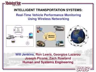
Spatial DBMS and Intelligent Transportation System Shashi Shekhar Intelligent Transportation Institute and Computer Science Department University of Minnesota shekhar@cs.umn.edu (612) 624-8307 http://www.cs.umn.edu/~shekhar http://www.cs.umn.edu/research/shashi-group/
Biography Highlights • 7/01-now : Professor, Dept. of CS, U. of MN • 12/89-6/01 : Asst./Asso. Prof. of CS, U of MN • Ph.D. (CS), M.B.A., U of California, Berkeley (1989) • Member: CTS(since 1990),Army Center, CURA • Author: “A Tour of Spatial Database” (Prentice Hall, 2002) and 100+ papers in Journals, Conferences • Editor: Geo-Information(2002-onwards), IEEE Transactions on Knowledge and Data Eng.(96-00) • Program chair: ACM Intl Conf. on GIS (1996) • Tech. Advisor: UNDP(1997-98), ESRI(1995), MNDOT GuideStar(1993-95 on Genesis Travlink) • Grants: FHWA, MNDOT, NASA, ARMY, NSF, ... • Supervised 7+ Ph.D Thesis (placed at Oracle, IBM TJ Watson Research Center etc.), 30+ MS. Thesis
Research Interests • Knowledge and Data Engineering • Spatial Database Management • Spatial Data Mining(SDM) and Visualization • Geographic Information System • Application Domains : Transportation, Climatology, Defence Computations
Spatial Data Mining, SDBMS • Historical Examples • London Cholera (1854) • Dental health in Colorado • Current Examples • Environmental justice • Crime mapping - hot spots (NIJ) • Cancer clusters (CDC) • Habitat location prediction (Ecology) • Site selection, assest tracking, spatial outliers
ITS Database Systems ITS Database Highway Based Sensor Drivers Home, office Shopping mall Information center, PCS Traffic Reports Road Maps City Maps Construction Schedule Business Directory Transportation Planners, Policy Maker
SDBMS & SDM in ITS • Operational • Routing, Guidance, Navigation for travelers and Commuters • Asset tracking in APTS, CVO for security, and customer service • Emergency services • Ramp meter control (freeway operation) • Incident management • Tactical • Event planning (maintenance, sports connection) • Infrastructure security - patrol routes • Snow cleaning routes and schedules • Impact analysis (e.g. Mall of America) • Strategic • Travel demand forecasting for capacity planning • Public transportation route selection • Policy decision(e.g. HOV lanes, ramp meter study) • Research: Driving Simulation and Safety
SDBMS and SDM in ITS • Transportation Manager • How the freeway system performed yesterday? • Which locations are worst performers? • Traffic Engineering • Where are the congestion (in time and space)? • Which of these recurrent congestion? • Which loop detection are not working properly? • How congestion start and spread? • Traveler, Commuter • What is the travel time on a route? • Will I make to destination in time for a meeting? • Where are the incident and events? • Planner and Research • How much can information technique to reduce congestion? • What is an appropriate ramp meter strategy given specific evolution of congestion phenomenon?
Transportation Projects • Traffic Database System • Traffic Data Visualization • Spatial Outlier Detection • Roadmap storage and Routing Algorithms • Road Map Accuracy Assessment • Other: • Driving Simulation • In-vehicle headup display evaluation
Project: Traffic Database System Sponsor and time-period: MNDOT, 1998-1999 Students: Xinhong Tan, Anuradha Thota Contributions to Transportation Domain Reduce response of queries from hours to minutes Performance tuning (table design, index selection) Contributions to Computer Science GUI design for extracting relevant summaries Evaluate technologies with large dataset
Gui Design • http://www.cs.umn.edu/research/shashi-group/TMC/html/gui.html
Flow of Data From TMC Storage at University of Minnesota Data made available for researchers FTP link TMC Server Binary ASCII FTP link FTP link PC FTP link Conversion programs Convert binary to 5min data
Existing Table Fivemin Detector ReadDate Time Dayofweek Volume Occupancy Validity Speed
Table Designs Fivemin Current Detector ReadDate Time Volume occupancy validity speed Day_week Fivemn_day Proposed-1 ReadDate Detector Vol_Occ_Validty Five_min Proposed-2 Detector Time_id Volume occupancy validity DateTime Time_id ReadDate Time Five_min MN/Dot Vol_5_ min Occl_5_ min Validity_5_ min Detector ReadDate Hour time 15mn 1hr Day_week Five_min Binary Detector ReadDate Time Volume occupancy validity
Benchmark Queries 1. Get 5-min Volume, occupancy for detector ID = 10 on Oct. 1st, 1997 from 7am to 8am 2. Get 5-min volume, Occupancy for detector ‘5’ on Aug1 1997. 3. Get 5-min volume, Occupancy for detector ‘5’ on Aug1 1997 from 6.30am to 7.30am. 4. Get average 5-min volume, occupancy, for Monday in Aug1997 between 8.00 - 8.05,8.05-8.10 …… 9.00 5. Get maximum volume, Occupancy for detector ‘5’ on Aug1 1997 from 6am to 7am 6. Get the average of AM rushhour hourly volume for a set of stations on highway I35W-NB with milepoint between 0.0 and 4.0 from Oct. 1st, 1997 to Oct. 5th , 1997 Conclusion
Examples of the Query • Example1: • Query description: • Get 5-min Volume, occupancy for detector ID = 10 on Oct. 1st, 1997 from 7am to 8am • SQL statement: • SELECT readdate, time, xtan.fivemin.detector, occupancy, volume • FROM xtan.fivemin, xtan.datetime • WHERE ReadDate = to_date('01-OCT-97', 'DD-MON-YYYY') • AND time BETWEEN '0705' AND '0800' • AND xtan.fivemin.Detector = '10' • AND xtan.fivemin.
Examples of the Query • Query result 1:
Examples of the Query • Example2: • Query description: • Get the average of AM rushhour hourly volume for a set of stations on highway I35W-NB with milepoint between 0.0 and 4.0 from Oct. 1st, 1997 to Oct. 5th , 1997 • SQL statement: • SELECT hour, xtan.v_stat_hour.station, avg(volume) • FROM tan.v_stat_hour, xtan.statrdwy • WHERE ReadDate BETWEEN to_date('01-OCT-97','DD-MON-YYYY') AND to_date('05-OCT-97','DD-MON-YYYY') • AND hour BETWEEN '06' AND '09' • AND statrdwy.route = 'I35W-I' • AND statrdwy.mp >= 0.0 • AND statrdwy.mp <= 4.0 • AND xtan.v_stat_hour.station = statrdwy.station • GROUP BY xtan.v_stat_hour.station, hour
Examples of the Query • Query result 2:
Conclusions • MN/Dot model and Proposed-II(Normalized) are the two recommended models for the final structure Proposed-II MN/Dot Conversioneffort Needs new loading program Little modification on existing loading process Same format remains Future Compatibility Number of columns increases Derived data Effort needed for derived data Fifteenmin & hourly data exist, station data needs to be derived Query More flexible Less flexible
Project: Traffic Data Visualization Sponsor and time-period: USDOT/ITS Inst., 2000-2001 Students: Alan Liu, CT Lu Contributions to Transportation Domain Allow intuitive browsing of loop detector data Highlight patterns in data for further study Contributions to Computer Science Mapcube - Organize visualization using a dimension lattice Visual data mining, e.g. for clustering
Motivation for Traffic Visualization • Transportation Manager • How the freeway system performed yesterday? • Which locations are worst performers? • Traffic Engineering • Where are the congestion (in time and space)? • Which of these recurrent congestion? • Which loop detection are not working properly? • How congestion start and spread? • Traveler, Commuter • What is the travel time on a route? • Will I make to destination in time for a meeting? • Where are the incident and events? • Planner and Research • How much can information technique to reduce congestion? • What is an appropriate ramp meter strategy given specific evolution of congestion phenomenon?
Dimensions • Available • TTD : Time of Day • TDW : Day of Week • TMY : Month of Year • S : Station, Highway, All Stations • Others • Scale, Weather, Seasons, Event types, …
Mapcube : Which Subset of Dimensions ? TTDTDWTMYS TTDTDWS TTDTDW TDWS STTD S TTD TDW Next Project
Singleton Subset : TTD Configuration: • X-axis: time of day; Y-axis: Volume • For station sid 138, sid 139, sid 140, on 1/12/1997 Trends: • Station sid 139: rush hour all day long • Station sid 139 is an S-outlier
Singleton Subset: TDW • Configuration: • X axis: Day of week; Y axis: Avg. volume. • For stations 4, 8, 577 • Avg. volume for Jan 1997 • Friday is the busiest day of week • Tuesday is the second busiest day of week Trends:
Singleton Subset: S Configuration: • X-axis: I-35W South; Y-axis: Avg. traffic volume • Avg. traffic volume for January 1997 Trends?: • High avg. traffic volume from Franklin Ave to Nicollet Ave • Two outliers: 35W/26S(sid 576) and 35W/TH55S(sid 585)
Dimension Pair: TTD-TDW Configuration: • Evening rush hour broader than morning rush hour • Rush hour starts early on Friday. • Wednesday - narrower evening rush hour • X-axis: time of date; Y-axis: day of Week • f(x,y): Avg. volume over all stations for Jan 1997, except Jan 1, 1997 Trends:
Dimension Pair: S-TTD Configuration: • X-axis: Time of Day • Y-axis: Highway • f(x,y): Avg. volume over all stations for 1/15, 1997 Trends: • 3-Cluster • North section:Evening rush hour • Downtown area: All day rush hour • South section:Morning rush hour • S-Outliers • station ranked 9th • Time: 2:35pm • Missing Data
Dimension Pair: TDW-S • X-axis: stations; Y-axis: day of week • f(x,y): Avg. volume over all stations for Jan-Mar 1997 • Busiest segment of I-35 SW is b/w Downtown MPLS & I-62 • Saturday has more traffic than Sunday • Outliers – highway branch Configuration: Trends:
Post Processing of cluster patterns • Clustering Based Classification: • Class 1: Stations with Morning Rush Hour • Class 2: Stations Evening Rush Hour • Class 3: Stations with Morning + Evening Rush Hour
Triplet: TTDTDWS: Compare Traffic Videos Configuration: Traffic volume on Jan 9 (Th) and 10 (F), 1997 • Evening rush hour starts earlier on Friday • Congested segments: I-35W (downtown Mpls – I-62); I-94 (Mpls – St. Paul); I-494 ( intersection I-35W) Trends:
Size 4 Subset: TTDTDWTMYS(Album) • Outer: X-axis (month of year); Y-axis (highway) • Inner: X-axis (time of day); Y-axis (day of week) Configuration: Trends: • Morning rush hour: I-94 East longer than I-35 W North • Evening rush hour: I-35W North longer than I-94 East • Evening rush hour on I-94 East: Jan longer than Feb
Project: Spatial Outlier Detection Sponsor and time-period: USDOT/ITS Inst. (2000-2002) Students: C T Lu, Pusheng Zhang Contributions to Transportation Domain Filter/reduce data for manual browsing Identify days with spatial outliers Identify sensors with anamolous behaviour Contributions to Computer Science Unified definition of spatial outliers using algebraic aggregates Spatial outlier detection algorithm = scan spatial join
Algorithms for Spatial outlier detection Spatial outlier A data point that is extreme relative to it neighbors Given A spatial graph G={V,E} A neighbor relationship (K neighbors) An attribute function f: V -> R Test T for spatial outliers Find O = {vi | vi V, vi is a spatial outlier} Objective Correctness, Computational efficiency Constraints Computation cost dominated by I/O op. Test T is an algebraic aggregate function
Spatial outlier detection Example Outlier Detection Test 1. Choice of Spatial Statistic S(x) = [f(x)–E y N(x)(f(y))] Theorem: S(x) is normally distributed if f(x) is normally distributed 2. Test for Outlier Detection | (S(x) - s) / s | > Hypothesis I/O cost = f( clustering efficiency ) f(x) S(x) Spatial outlier and its neighbors
Spatial outlier detection Results 1. CCAM achieves higher clustering efficiency (CE) 2. CCAM has lower I/O cost 3. Higher CE leads to lower I/O cost 4. Page size improves CE for all methods CE value I/O cost Cell-Tree CCAM Z-order
Project: Roadmap storage and Routing Algorithms Sponsor and time-period: FHWA/MNDOT, 1993-1997 Students: Prof. Du-Ren Liu, Dr. Mark Coyle, Andrew Fetterer, Ashim Kohli, Brajesh Goyal Contributions to Transportation Domain CRR = measure of storage methods for roadmaps In-vehicle navigation devices, routing servers on web Contributions to Computer Science CCAM - Better storage method for roadmaps Hierarchical routing - optimal routes even when map-size > memory size
Road Map Storage - Problem Statement • Given roadmaps • Find efficient data-structure to store roadmap on disk blocks • Goal - Minimize I/O-cost of operations • Find(), Insert(), Delete(), Create() • Get-A-Successor(), Get-Successors() • Constraint • Roadmaps larger than main memories
Mpls map partitioning 1 Another way that we may partition the street network for Minneapolis among disk blocks for improving performance of network computations.
Mpls map partitioning:CCAM This is one way that we may partition the street network for Minneapolis among disk blocks for improving performance of network computations.
Road Map Storage • Insight: I/O cost of network operations is minimized by maximizing • CRR = Pr. ( road-intersection nodes connected by a road-segment edge are together in a disk page) • WCRR = weighted CRR (edges have weights) • Commercial database support geometric storage methods even though CRR is a graph property
Shortest Path Problem • Route computation • Find a rout from current location to destination • Criteria: Shortest travel distance or smallest travel time • Useful for • Travel during rush hour • Travel in an unfamiliar area • Travel to an unfamiliar destination
Problem definition • Given • Graph G=(N,E,C) • Each edge (u,v) in E has a cost C(u,v) • Path from source to destination is a sequence of nodes • Cost of path=C(vi-1,vi) • A path cost estimation is a function f(u,v) that computes estimated cost of an optional path between the two nodes
Smallest Paths Blue: Smallest travel time path between two points. It follows a freeway (I-94) which is faster but not shorter in distance. Red: Shortest distance path between the same two points
Algorithm for Single pair Path Computation • Road Map Size<<Main Memory Size • Iterative Algorithm • Dijkstra’s Algorithm • A* algorithm • A* with euclidean distance heuristic • A* with manhattan distance heuristic • Road Map Size >> Main Memory Size • Traditional algorithm run into difficulties! • Hierarchical Algorithm
Motivation for Hierarchical Algorithms • Road Map Size >> Main Memory Size • Traditional algorithms yield sub-optimal path • Heuristics - bounding box (source, destination) or Freeway first then sideroads • Example: Microsoft Expedia • route(Tampa FL to Miami, FL via Canada) • Need an algorithm to give optimal route • A piece of roadmap in memory at a time • Intuition - travelling from island to island
Hierarchical Routing : Step 1 • Step 1: Choose Boundary Node Pair • Minimize COST(S,Ba)+COST(Ba,Bd)+COST(Bd,D) • Determining Cost May Be Non-Travial