Download
1 / 23
230 likes | 392 Views
Dynamics of wind-forced coherent anticyclones in the open ocean. Inga Koszalka, ISAC-CNR, Torino, Italy Annalisa Bracco , EAS-CNS, Georgia Tech Antonello Provenzale, ISAC-CNR, Torino, Italy. Idealized set-up to investigate the dynamics of wind-driven coherent anticyclones in the open ocean.

E N D
Dynamics of wind-forced coherent anticyclones in the open ocean Inga Koszalka, ISAC-CNR, Torino, Italy Annalisa Bracco, EAS-CNS, Georgia Tech Antonello Provenzale, ISAC-CNR, Torino, Italy
Idealized set-up to investigate the dynamics of wind-driven coherent anticyclones in the open ocean • Double-periodic domain • Constant depth H=1000m; lateral size L=256Km or L=128Km • Resolution Δx=1 km, 18 and 80 vertical layers (6 and 27 in the first 100 meters) • Coriolis frequency f = 10-4s-1 • Narrow band wind forcing kx = ky = 6 (Muller & Frankigoul 1981), withan added random noise component: τx (x, y) = 0.1 * sin(2πkx x) sin(2πky y) + 0.3 (ran[0-1]- 0.5)
temperature profile T(z) =10+12exp(0.017 z) oC and salinity S(z) = 35+2.0 exp(0.024 z) PSU (WOA, 2001) • costant solar shortwave radiation: QT = 150 W=m2 (Hatzianastassian et. al. 2005, for mid-latitudes in April) • Lagrangian tracers: released after the system had achieved a statistically stationary state in the 18-layers run in 3 sets of 4096 floats at -1, 78 and 204m on a regular grid • The system, under the assumption of being equivalent barotropic, is characterized by the following Rossby, Froude number and Rossby deformation radius:
Spin-up phase: the nonlinear spin-up circulation establishes in the form of symmetrical Ekman-circulation cells, which scales are related to those of the forcing (so not generic). Following the nonlinear Ekman circulation theory, the anticyclonic patches grow stronger due to positive feedback between Ekman transport and anticyclonic vorticity (e.g. Niiler 1969). • Around ~ day 25 the vortices form, which is of the order of the characteristic spin-up time for the system defined as (Pedlosky, 1987) • From this time on, the system is characterized by the presence of coherent structures of different scales (of the size of initial circulation cells or smaller). Predominantly anticyclones, shielded by rings of positive undergoing continuous formation, decay and merging • The nudging to the temperature and salinity profiles prevents the system from barotropization
Cyclones/anticyclones asymmetry Cushman-Rosin & Tang 1990: stability argument suggesting that, on a f -plane, in the presence of the free surface, axis-symmetric vortices are solutions that optimize the kinetic energy, but while the anticyclonic vortices are stable, cyclones are not Polvani et al., 1994: the asymmetry increases with Fr (i.e. with the importance of the free-surface effect) and cyclones correspond to contractions of the fluid layer (negative free surface, η< 0). Additionally anticyclones are internally more coherent and merge (grow) more easily as the range of interaction within each vortex is larger than for cyclones of comparable relative vorticity Thomas and Rhines, 2002: positive feedbacks between Ekman transport and negative vorticity when rotational surface is present Graves et al., 2005, 2006: The controlling mechanisms in Shallow Water systems is vortex weakening under straining deformation, with the weakening being substantially stronger for cyclones than anticyclones. The outcome is a strain-induced vortex weakening of cyclones in particular when the deformation radius is not large compared to the vortex radius and the Rossby number is not small
Top: Vertical component of normalized relative vorticity ζ/f at the surface (left) and at 78m depth (right). It provides an estimate of the local value of the Rossby number. Bottom: Vertical velocity in m/day at 78m depth (left); vertical section of vertical velocity (in m/day) across the line indicate above
Horizontal motion 2D power spectra of kinetic energy as function of depth we do not have a mixed layer! However…
From Rupolo et al, JPO, 1996: Power spectra from floats in the Western North Atlantic at 700m depth
in the model Horizontal velocity distributions Western North Atlantic z < 1000m from Bracco et al., JPO, 2000
what are the components contributing to the vertical velocities?
profile of standard deviation of the vertical velocity from ROMS and calculated from formula
Profile of the std of the contribution of different terms to the vertical velocity (integrated in the vertical). Note the logarithmic scale.
The distributions of vertical velocities are non-Gaussian at all depths and vertical velocities strongly impact the vertical displacement of Lagrangian tracers
Example trajectories of initially close-by particle pairs released at 78m (top) and at the surface (right)
conclusions • We analyzed idealized runs with wind-forced vortices when the internal Rossby deformation radius is small with respect to the domain size, resulting in the generation of surface intensified coherent anticyclones. • In the upper 150 meters of the water column, the vortical motion dominates over the divergent component, near-inertial waves are negligible and most statistical properties of horizontal flows (apart from the cyclone-anticyclone asymmetry) are similar to those of barotropic and QG turbulence, including hor. velocity distributions and absolute and relative dispersion
The vertical velocity field is complex and cannot be described by simpler models. Vertical velocities can reach instantaneous values of up to 100 m/day and display a fine spatial structure • Upwelling and downwelling regions alternate and do not correlate with relative vorticity but result from the interplay of advection, stretching and instantaneous vorticity changes • The primary balance is attained by ageostrophic and stretching terms (O(100m/day));The tilting term contribution is of O(10m/day) at the surface and declines with depth. Free-surface, rotation of the wind stress and mixing terms are smaller by three to four orders of magnitude, depending on depth • All terms are modulated by (f +ζ)−1 , which can be large inside anticyclones where |ζ| ~f and ageostrophic effects arise. This explains why there is no simple correlation between vertical velocities and the vorticity field or its gradients
finally… is this of any relevance? At least for lab experiments seems so… courtesy of John Wettlaufer and Michael Patterson
Figures in slide before show the development of a vortex and the complete vortex in a lab experiment and are constructed from 3D PIV series of horizontal slices. There is a free surface and an Ekman layer at the bottom. The structure of the vertical velocity field is as in our runs (ask John for images) And in chlorophyll distributions inside anticyclones (McGillicuddy et al., 2007, Science)