Download
1 / 28
280 likes | 505 Views
Agricultural and Urban Water Use Scenario Evaluation Tool. California Water Plan Update 2004. Conceptual Framework. Demand Drivers. Geophysical Parameters. Water Management Objectives. Water Management System. Human and Environmental Water Demands. Management Options.

E N D
Agricultural and Urban Water Use Scenario Evaluation Tool California Water Plan Update 2004
Conceptual Framework Demand Drivers Geophysical Parameters Water Management Objectives Water Management System Human and Environmental Water Demands Management Options Evaluation Criteria (Economic, Management, Societal) Overview Organization Definitions
Irrigated crop area Irrigated land area Crop unit water use Mix of annual and permanent crops Ag WUE Irrigated land retirement Total Population Population density Population distribution Commercial activity Industrial activity Urban WUE Naturally occurring conservation Scenario factors that influence ag and urban water use
Ag and Urban Water Use Scenario Evaluation Tools • Sensitivity analysis • Quantification of uncertainty • Informed by more-sophisticated models • Interact with other tools as modules in an analytical environment • Analytical environment accounts for the entire flow diagram
Ag Water Use Initial Condition Scenario Crop ET Crop ET Crop ET Informed by ETAW Model, SIMETAW, CALAG, and other sources Effective Precip Effective Precip EP ETAW ETAW Consumed Fraction Consumed Fraction CF Unit Applied Water Unit Applied Water Informed by ETAW Model, California Land and Water use data base, Water Portfolios, and other sources Irrigated Crop Area ICA Irrigated Crop Area Irrigated Land Area ILA Irrigated Land Area Applied Water Applied Water
Urban Water Use Initial Condition Scenario WU by Sector Drivers Housing Units Persons/HH HH Income Water Price Employment Urban WUE Informed by IWR-MAIN, CUWA Study, PI Study, and other sources Drivers Housing Units Persons/HH HH Income Water Price Employment Urban WUE Drivers Unit Water Use SFR Unit MFR Unit Comm. employee Ind. employee Per person Unit Water Use SFR Unit MFR Unit Comm. employee Ind. employee Per person Informed by IWR MAIN, Water Portfolios, and other sources Unmodified WU by Sector
Traditional Spreadsheet Approach • Combination of single “point” estimates to predict a single result • Can reveal sensitivity of dependent variables to change in model inputs • Based on estimates of model variables • Single estimate of results, i.e, cannot assess uncertainty inherent in model inputs
Simulation Approach • Technical and scientific decisions all use estimates and assumptions • The simulation approach explicitly includes the uncertainty in each estimate • Results reflect uncertainty in input variables
Scenario Evaluation Tools in an Analytical Environment • Multiple screening tools to serve various purposes • Ag water use • Urban water use • Water supplies • Water management options • Each informed by more-sophisticated models • Readily reveal sensitivity and uncertainty introduced through changes to model inputs. • Housed as modules in a common analytical environment governed by a standard set of rules – Analytica, STELLA, Extend, Vensim
Why Use an Analytic Environment? • Communicate model structure • Integrate documentation • Ease of review and audits • Collaboration • Facilitate hierarchical structure • Manage complexity • Permit refinement and desegregation • Exploration of uncertainty effects Adapted from: Granger and Henrion. 1990. Uncertainty, A Guide to Dealing with Uncertainty in Quantitative Risk and Policy Analysis, Cambridge University Press.
The Analytica Modeling Environment • Uses Influence Diagrams • Nodes • Decision variables • Chance variables • Deterministic Variables • Arcs • Indicates dependence or influence between nodes • Uses a Hierarchical Structure • More info at www.lumina.com • Other environments similar
Built in tools address uncertainty in several ways • Probabilistically • Assign probability functions to variables • View results probabilistically • Parametrically • Explore the space of outcomes • Pick individual parameters to define a scenario
Easy, built in displays and user interface facilitate understanding • Quick graphs of variables • Change key variables within graphing window or control panel • Imbedded documentation for all elements
Water Plan Narrative Scenarios Quantified Using Analytica-based Model • Urban and Agricultural Demand • Based primarily on DWR’s spreadsheet models • Estimates for each hydrologic region • Variable time-step • Initial conditions based on 2000 data
Urban Water Demand Calculated Using Bottom-Up Approach • Demand Units • Households • Single- and multi-family • Interior and Exterior • Commercial Employees • Industrial Employees • Institutional Use (per capita)
Residential Sector Population SF & MF Homes Household Size Indoor and Outdoor WU Public / Institutional Sector Population Public WU Commercial and Industrial Sectors Population Commercial & Industrial Employment Commercial & Industrial WU Model is Initialized with Year 2000 Data
Population Changes DriveHousing and Employment • SF and MF houses a function of: • Population • Fraction of population houses • Share of SF houses • Household Size • Com. & Indust. employees a function of: • Population • Employment rate • Commercial Job Fraction • Commercial Jobs/(Commercial + Industrial Jobs)
Per unit water demand(water use coefficient) • Many factors can influence water use coefficient (WUC) • Simplest approach • Percentage change in WUC for each sector • Easy interpretation • In future, disaggregate effects • Income, water price, naturally occurring conservation, water use efficiency • Permit more permutations for other scenarios
Irrigation Demand Calculated by Estimating Crop Demand • IU=State-wide irrigation water use • ICA=Irrigated crop area • Irrigated Land Area + Multi-cropped Area • AW=Required applied water per area for each crop
Required Water for Crops • For each crop and HR: AW = ETAW / CF where ETAW = Evapotranspiration – Effective Precipitation CF = Consumed Fraction CF ranges from ~55% for Rice to ~80% for tomatoes
Irrigation demand changeover time • IU changes if any of the following change: • ILA – change in irrigated land area • MA/ILA – change in ratio of multi-cropped area • AW – improved varieties of crops, better irrigation methods or technology, change in weather • Cropping pattern – currently implemented as change in AW
Environmental Demand • Based on Environmental Defense memo (Dec. 8, 2003) • 2000 Unmet demand: