Learn how to make your drawings come alive…

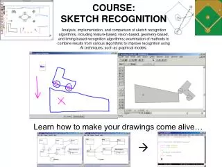
1.  COURSE: SKETCH RECOGNITION Analysis, implementation, and comparison of sketch recognition algorithms, including feature-based, vision-based, geometry-based, and timing-based recognition algorithms; examination of methods to combine results from various algorithms to improve recognition using AI techniques, such as graphical models. Learn how to make your drawings come alive…

2. Gesture Recognizers?

3. Rubine Long Discussion

4. Paulson Review

5. Sezgin Corner Finding Algorithm • Finds corners in a polygon or in a complex shape.

6. Implications • By finding corners, • You can build objects geometrically • Users can use multiple strokes

7. Claim to Fame • This algorithm was the first to notice that corners were identifiable not only be curvature, but also by speed. • The pen slows down when you ‘intend’ to make a corner.

8. Algorithm Overview • Find corners based on curvature alone • Find corners based on speed alone • Find intersection • Add one extra corner at a time until error is below threshold.

9. Direction Graph Direction of each stroke segment = arctan2(dy,dx) Add check to make sure graph continuous (e.g., add 2pi)

10. Curvature Graph Change in direction for each segment

11. Speed Graph Speed of each segment (already computed in Rubine)

12. Curvature Threshold • The threshold is set to the mean curvature

13. Speed Threshold • The threshold is set to 90% of the mean.

14. Select Curvature Vertices • Max of all sections above threshold • Fd = curvature points

15. Select Speed Vertices • Max of all sections below threshold • Fs = speed points

16. Initial Fit • You now have a list of curvature corners: Fd • And a list of speed corners: Fs • The initial fit is the Intersection of Fd and Fs - (and of course the endpoints) • (Note that now the candidate corners are limited to Fs union Fd)

17. Improving Fit • We check the error, if it is small enough, we stop, but if not, we want to try to add a vertex • Want to add one vertex at a time • Which do we add? • We try one curvature vertex • We try one speed vertex

18. Picking the Curvature Vertex to Add • Pick the vertex with the highest curvature • CCM(vi) = Curvature Certainty Matrix at vertex I • Compute CCM for each vertex candidates in Fd • Average-based filtering • Find curvature at vertex i using a neighborhood • CCM(vi) = di-k – di+k /l • di = curvature at vertex I • l = length of substroke from vi-k to vi+k • Note: thie is not Euclidean distance – even though variable in paper is used to mean this later.

19. What is k? • K is neighborhood size = number of stroke points on either side to search • Paper does not specify. • Suggestions: • Set k = 3 … AND / OR • Set k to the minimum value such that li is greater than 6 pixels

20. Picking the Speed Vertex to Add • Pick the slowest vertex • SCM(vi) = Speed Certainty Metric at stroke point i. • SCM(vi) = 1 – speedi / speedmax • Compute SCM for all speed vertex candidates (Fs) • Note: paper uses v for speed and vertex

21. Vertex Possibilities: • Fd: Possibilities based on curvature • Fs: Possibilities based on speed • CCM(Fd) : Curvature Certainty Metric • Used to rank Fd candidates • SCM(Fd) : Speed Certainty Metric • Used to rank Fs candidates • Remember: • H0 = Initial Hybrid Fit = intersection of Fd and Fs (and endpoints)

22. Improving Fit • Compute Error for H0 • If error below threshold stop… else • Add vertex with largest SCM (speed) not already chosen • Hi’ = H0 + max(SCM(Fs – H0) ) • Add vertex with largest CCM (curvature) not already chosen • Hi’’ = H0 + max(CCM(Fd – H0)) • Compute error for Hi’ and Hi’’ • Add the vertex that created the smaller error • You have only added one vertex • Repeat

23. Create Line Segments for Fit Approximation • For each vertex vi in Hi – create a list of line segments between vi and vi+1 • If there are n points in the vertex selection, there will be n-1 line segments

24. Measuring Fit Error • S = total stroke length (not Euclidean distance) • ODSQ = orthogonal distance squared • ODSQ(s,Hi) = distance of stroke point s to appropriate line segment (previous slide)

25. Distance from point to line segment • if isPointOnLine(point, line) • theDistance = 0; • else • array1 = getLineAxByC(line); • array2 = getAxByCPerpendicularLine(line, point); • A = [array1(1), array1(2); array2(1), array2(2)]; • b = [array1(3); array2(3)]; • intersectsPoint = linsolve(A, b)'; • if isPointOnLine(intersectsPoint, line) • theDistance = getLineLength([intersectsPoint; point]); • else • dist(1) = getLineLength([line(1,:); point]); • dist(2) = getLineLength([line(2,:); point]); • theDistance = min(dist); • end • end

26. What is the Error Threshold? • Stop when error is below the threshold. • … what is threshold? • Not in paper • Your choice: Suggestion: • Compute the error for H0 = e0 • Compute the error for Hall (all the chosen v) = eall • We want something in the middle: close to eall • .1*(e0-eall) + eall • You will try other thresholds in your implementation

27. Final Fit • Final fit is a polyline fit. • We have not yet created the complex fit.

28. Creating the Complex Fit • Stroke between corners can be curve or line • Compute euclidean distance (l1) / substroke length (l2) • L1/l2 • Is <= 1 (because l1 < l2) • If is close to 1, it is a line, else a curve • Paper leaves threshold to you: • Suggestion: .9 < l2/l1

29. Homework • Find corners using Sezgin method • Identify if substrokes between corners are lines or curves/arcs using distance metric

30. Sezgin Bezier Curve Fitting • Want to replace with a Bezier curve • http://www.math.ubc.ca/people/faculty/cass/gfx/bezier.html • Bezier Demo • 2 endpoints and 2 control points

31. Sezgin Bezier Curve Fitting • Control Point Approximation • c1 = k*t1 + v • c2 = k*t2 + u • Notation: • Endpoints: u = p1, v = p2 • T1= tangent vector – initial direction of stroke at point p1 (u) • T2 = tangent vector of p2 (v) – initial direction of stroke at point p2 • K = stroke length / 3 • 3 is common approximation

32. To test curve error: • Breaks into linear curves. • If error to great, splits curve in half (by stroke point – not distance)

33. Bezier curve equation • http://www.cl.cam.ac.uk/Teaching/2000/AGraphHCI/SMEG/node3.html • http://www.moshplant.com/direct-or/bezier/math.html • P0 (x0,y0) = p1, P1 = c1, P2 = c2, P3 = p2 • x(t) = axt3 + bxt2 + cxt + x0 • y(t) = ayt3 + byt2 + cyt + y0 • cx = 3 (x1 - x0)bx = 3 (x2 - x1) - cxax = x3 - x0 - cx - bx • cy = 3 (y1 - y0)by = 3 (y2 - y1) - cyay = y3 - y0 - cy - by

34. Circles and Ellipses • Least squares fit • Make a bounding box of stroke and form • Oval is formed from that bounding box. • Circle is easy: • Find out how far the circle is from the center = d, return (d-r)^2 • Ellipse more complicated

35. Improvement Ideas • Instead of testing the error, we test the improvement, if it is great enough, we add the vertex