Download
1 / 56
560 likes | 565 Views
Threshold Phenomena and Fountain Codes. Amin Shokrollahi. EPFL Parts are joint work with M. Luby, R. Karp, O. Etesami. BEC(p 1 ). BEC(p 2 ). BEC(p 3 ). BEC(p 4 ). BEC(p 5 ). BEC(p 6 ). Communication on Multiple Unknown Channels. Example: Popular Download. Example: Peer-to-Peer.

E N D
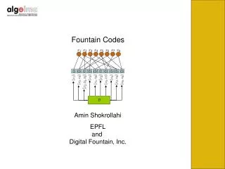
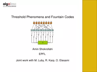
Threshold Phenomena and Fountain Codes Amin Shokrollahi EPFL Parts are joint work with M. Luby, R. Karp, O. Etesami
BEC(p1) BEC(p2) BEC(p3) BEC(p4) BEC(p5) BEC(p6) Communication on Multiple Unknown Channels
The erasure probabilities are unknown. Want to come arbitrarily close to capacity on each of the erasure channels, with minimum amount of feedback. Traditional codes don’t work in this setting since their rate is fixed. Need codes that can adapt automatically to the erasure rate of the channel.
Users reconstruct Original content as soon as they receive enough packets Original content Encoded packets Encoding Engine Transmission What we Really Want Reconstruction time should depend only on size of content
Content Enc Digital buckets
Content Server 1 Server 2 Reception from multiple servers Applications: Multi-site downloads
Sender 2 Sender 3 Rec 1 Rec2 Rec 3 Applications: Peer-2-Peer Sender 1
Fountain Codes Sender sends a potentially limitless stream of encoded bits. Receivers collect bits until they are reasonably sure that they can recover the content from the received bits, and send STOP feedback to sender. Automatic adaptation: Receivers with larger loss rate need longer to receive the required information. Want that each receiver is able to recover from the minimum possible amount of received data, and do this efficiently.
Fountain Codes Fix distribution on , where is number of input symbols. For every output symbol sample independently from and add input symbols corresponding to sampled subset.
Distribution on Fountain Codes
Universality and Efficiency [Universality] Want sequences of Fountain Codes for which the overhead is arbitrarily small [Efficiency] Want per-symbol-encoding to run in close to constant time, and decoding to run in time linear in number of output symbols.
Overhead is the fraction of extra symbols needed by the receiver as compared to the number of input symbols (i.e. if k(1+ε) is needed , overhead =ε) – want to be arbitrarily small Cost of encoding and decoding – linear in k Ratelessness – the number of output symbols is not determined apriori Space considerations (less important) Parameters
LT-Codes • Invented by Michael Luby in 1998. • First class of universal and almost efficient Fountain Codes • Output distribution has a very simple form • Encoding and decoding are very simple
LT-codes use a restricted distribution on : Fix distribution on Distribution is given by where is the Hamming weight of Parameters of the code are LT-Codes
Choose weight Prob Weight 1 0.055 2 0.3 Weight table 3 0.1 4 0.08 100000 0.0004 The LT Coding Process Input symbols Choose 2 Random original symbols XOR 2 Insert header, and send
Average Degree of Distribution should be Not covered Prob. Decoding error Prob. Non-coverage Ω’(1) = average output node degree
Average Degree of Distribution should be Not covered Luby has designed universal LT-codes with average degree around and overhead i.e. the number of symbols needed is
So: Average degree constant means error probability constant How can we achieve constant workload per output symbol, and still guarantee vanishing error probability? Raptor codes achieve this!
Use 2 phases: pre-code encodes k input symbols into intermediate code Apply LT to encode the intermediate code and transmit The LT-decoder only needs to recover (1-δ)n of the intermediate code w.h.p. This only requires constant degree! Raptor Codes
Input symbols d – fraction erasures Output symbols Raptor Codes Traditional pre-code LT-light
Not covered Redundant Checks If pre-code is chosen properly, then the LT-distribution can have constant average degree, leading to linear time encoding. Raptor Code is specified by the input length , precode and output distribution . How do we choose and ? Raptor Codes X
Special Raptor Codes: LT-Codes LT-Codes are Raptor Codes with trivial pre-code: Need average degree LT-Codes compensate for the lack of the pre-code with a rather intricate output distribution.
Max degree Degree distribution: Average Degree: W.h.p can decode LT-lite
Can use regular LDPC codes such as Tornado, right-regular code, etc. But they have high average degree distributions… What about pre-code?
An LDPC code can be systematic (I.e. input symbols appear in the set of the output symbols) Code rate (k/n) is arbitrarily close to 1, so most intermediate symbols have degree 1 Key Point
Encoding and Decoding can be done in time linear in k (or constant time per input symbol) The overhead is arbitrarily small as in regular LT codes Storage requirement is just the stretch factor n/k and k is arbitrarily close to n Conclusions
Progressive Giant Component Analysis A different method for the analysis of the decoder: Want enough nodes of degree 2 so there exists a giant component in the induced (random) graph on input symbols.
Progressive Giant Component Analysis First giant component removes -fraction of input symbols. Residual distribution: Fraction of residual nodes of degree 2: Average degree of new induced graph: Condition: “Ideal distribution:”
Progressive Giant Component Analysis Analysis does not use “tree-assumption”, but only properties of induced graph. Analysis can be used to obtain error bounds for the decoding algorithm. It can also be used to obtain capacity-achieving distributions on the erasure channel. A modified version can be used to obtain for capacity-achieving distributions for other symmetric channels.
New output node of degree 2 Nodes of Degree 2 Information Loss!
If there exists component of linear size (i.e., a giant component), then next output node of degree 2 has constant probability of being useless. Therefore, graph should not have giant component. This means that for capacity achieving degree distributions we must have: On the other hand, if then algorithm cannot start successfully. So, for capacity-achieving codes: Fraction of Nodes of Degree 2
The -ary symmetric channel (large ) Double verification decoding (Luby-Mitzenmacher): If and are correct, then they verify . Remove all of them from graph and continue. Can be shown that number of correct output symbols needs to be at least Times number of input symbols.
The -ary symmetric channel (large ) More sophisticated algorithms: induced graph! If two input symbols are connected by a correct output symbol, and each of them is connected to a correct output symbol of degree one, then the input symbols are verified. Remove from them from graph.
The -ary symmetric channel (large ) More sophisticated algorithms: induced graph! More generally: if there is a path consisting of correct edges, and the two terminal nodes are connected to correct output symbols of degree one, then the input symbols get verified. (More complex algorithms.)
The -ary symmetric channel (large ) Limiting case: Giant component consisting of correct edges, two correct output symbols of degree one “poke” the component. So, ideal distribution “achieves” capacity.