Download
1 / 12
120 likes | 187 Views
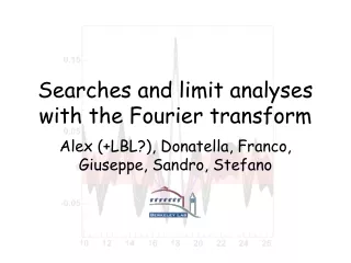
Searches and limit analyses with the Fourier transform. Alex, Amanda, Donatella, Franco, Giuseppe, Hung-Chung, Johannes, Juerg, Marjorie, Sandro, Stefano. Outline. Reminder of method Example Task list Status: “Fitter” More details on individual issues in other talks:

E N D
Searches and limit analyses with the Fourier transform Alex, Amanda, Donatella, Franco, Giuseppe, Hung-Chung, Johannes, Juerg, Marjorie, Sandro, Stefano
Outline • Reminder of method • Example • Task list • Status: • “Fitter” • More details on individual issues in other talks: • Mass fit (Hung-Chung) • Extraction of ct curves (Amanda) • ct scale factor (Aart, Amanda) • Samples & Skimming (Marge)
The Method • We are looking for a periodic signal: Fourier space is the natural tool • Moser and Roussarie already mentioned this! • They use it to derive the most useful properties of A-scan • Amplitude approach is approximately equivalent to the Fourier transform Amplitude from scan Re[Fourier] • Aim: move to Fourier transform based analysis • Computationally lighter • As powerful as A-scan • As is, no need *in principle* for measurements of D, etc. (however these ingredients add information and tighten the limit) • Will provide an alternate path to the A-scan result!
Dilution weighted transform • Discrete Fourier transform definition • Given N measurements {tj} • Properties: • A particular application of (CDF8054) • Average: • (f(t) is the parent distribution of {tj}) • Corresponds to dilution-weighted Likelihood approach • Errors computed from data: • NB: Errors can be calculated directly from the data! • behaves “as you’d expect” • While and its uncertainty are fully data-driven, predicted requires exactly the same ingredients as the amplitude scan fit
Properties of … • Re[] • contains all the information of the standard amplitude scan • Amplitude scan properties are mostly derived assuming: (Amplitude scan)Re[] • Re[F] and Re[F]can be computed directly from data! • b) Sensitivity is exactly: Can we reproduce the A-scan itself?
Toy Example “A-scan” a` la fourier • 1000 toy events • ms=18 • S/B=2. • Dsignal2=1.6% • Dback2=0.4% • Background and signal parameterized according to standard analyses • Histogrammed ct • Best knowledge on SF parameterization Sensistivity: Predicted Measured No actual fit involved: this method allows to flexibly study systematics!
Plans for our method • Final proof of principle: Process all data from last round of analyses and show consistent picture with standard A-scan • Prove viability of our method: • Full semileptonic and hadronic samples • Same taggers and datasets as latest blessed A-scans • Compare results to our method • Will be ready on time for winter conferences • Extend: • 1fb-1 • All possible modes • State of the art taggers • We will have a full analysis by Summer conferences
Ntuples & Skim • All modes being analyzed, started from the easiest for cross checks • Old sample used as benchmark, based on last round of mixing results • Satisfactory comparison so far (see histogram on right) • Minor discrepancies: • Missing upper mass sideband: will fix • Ready for prime time! • (you’ll see results on new data from Marge & Amanda)
Fitter Status • “Fitter” fully implemented • Provided in the same consistent framework: • Data processing • Toy MC generation • Bootstrap extraction • Combination of several samples Pulls Mean vs Pulls vs
Fitter performance: Amplitude scan on old data • Already unblinded (355 pb-1) • Model (D, ct etc.) from the same sample • Ds[] alone • All taggers included • Fitter works! • Next steps: • Infrastructure to combine samples (almost ready) • Point-by-point comparison with a ‘fitted’ amplitude scan Clean up and move to semileptonics!
Tasks (my view, still being finalized not yet endorsed/discussed) • Data [Donatella, MDS, Stefano] • Skimming, event by event comparison with MIT sample [Donatella, Marjorie] See Marge’s talk • MC [Hung-Chung+JHU] See HC’s talk on mass fits etc. • Ntuples [Johannes, Giuseppe] • Reco: [Alex,MDS, Stefano] • Optimize selections [Alex, MDS] • New channels (new modes, partially reconstructed) [Alex, MDS] • Basic tools: [Stefano, Alex, MDS, Giuseppe, Johannes] • PID [Stefano] • Vertexing (understand resolutions etc.) [Alex, Amanda, MDS] • new taggers? (OSKT, SSKT...) [Giuseppe, Johannes] • Efficiency curves [Amanda] • Ct resolution & scale factors [Alex, Amanda, Marge] See Amanda’s talk • Fourier “fitter” [Alex, Franco] • Toy MC [Alex, Franco] This talk • Tool for data Analysis (from ct, sigma, D, etc. to “the plot”) [Alex, Franco] • Semileptonic Analysis [Alex, Sandro] • Spring Analysis: reproduce the MIT result • Summer Anal.: - full 1 fb-1 indipendent analysis • Hadronic Analysis (same as 5) [Alex, Amanda, Giuseppe, Hung-Chung, Stefano] • Combine Analyses [Alex]
Conclusions • This is an AGGRESSIVE PLAN • Good progress in the last 2 months • We need to keep going, faster? • We want to have • Reproduce blessed results by March (Moriond) • independent results by the summer!