Download
1 / 90
920 likes | 1.19k Views
Genomics. Irena Artamonova. Second European School of Bioinformatics Nijmegen, January 22, 2005. Complete genomes. Brief calculation. Approximately 233 complete genomes with about 3000 genes in each on average. Almost all genes are new and unstudied

E N D
Genomics Irena Artamonova Second European School of Bioinformatics Nijmegen, January 22, 2005
Brief calculation Approximately 233 complete genomes with about 3000 genes in each on average. Almost all genes are new and unstudied In a lab: investigation of function of one gene requires one postdoc-year at least. Hurrah!: we have work for all molecular biologists for thousands of years right now!
We have a new “complete genome”. What can we do with it now (in silico)?(outline of the lecture) Gene recognition Prediction of regulation of gene expression Functional annotation of proteins Metabolic reconstruction Study of genome evolution Main differences: Prokaryotes and Eukaryotes
Size of a prokaryotic genome: Pathogenesis bacteria - from < 1 Mb and 600 genes Free living bacteria – up to 6-9 Mb, 9000 genes Gene recognition I. Prokaryotes E.g., Escherichia coli: 4.6 Mb - 4400 генов Projection of known genes Genome comparisons Finding long ORFs Using DNA statistics Identification of gene starts
Mapping “known” genes BLASTx: //www.ncbi.nlm.nih.gov/BLAST/ A lot of information when a close genome is well-studied. But it happens rarely. Problems: choice of thresholds, fine mapping of start positions in other cases. No perfect solutions.
Using long ORFs • What minimal length is functional? • Which Met is the start? ORFs in a fragment of the K. pneumoniae genome
Use of DNA statistics in gene recognition Frequencies of codons differ from frequencies of non-coding triplets: frequencies of amino acids (and their) codons; frequencies of dipeptides; frequencies of synonymous codons (genome-specific, correlate with tRNA concentration).
Coding potential • “Sliding window” technique: • Scan the DNA sequence with sliding window of fixed size • Calculate coding potential for each window position and plot it above the sequence (horizontal axis) • Choosing of a window size so as to minimize random noise A function measuring whether the genomic fragment is coding or non-coding based on its DNA statistics. We can calculate coding potential for ORFs or for sliding window
Selection of window size for sliding window E. coli: 96nt window 48nt window
Exact mapping of gene start positions • Prokaryotes: starting methionine is preceded by a ribosome-binding site (so-called Shine-Dalgarno box, any part of GGAGGA) • Extension of the nucleotide alignment with orthologous region from a related genome: mutation patterns in the coding region differ from the those in the intergenic region
rbsD in enterobacteria Sty AGGGTTACACTGCGGC-CAGCGAAACGTTTCGCTAGTGGAGCAGAAAAATGAAGAAAGGC Sen AGGGTTACACTGCGGC-CAGCGAAACGTTTCGCTAGTGGAGCAGAAAAATGAAGAAAGGC Stm GGGGTTACACTGCGGC-CAGCGAAACGTTTCGCTAGTGGAGCAGAAAAATGAAGAAAGGC Eco AGGATTAAACTGTGGGTCAGCGAAACGTTTCGCTGATGGAGAA-AAAAATGAAAAAAGGC Ype TTTTCTAAACTCCTTGTTAGCGAAACGTTTCGCTCTTGGAGTA-GATCATGAAAAAAGGT ** *** **************** ***** * * ***** ***** Sty ACCGTACTCAACTCTGAAATCTCGTCGGTCATTTCCCGTCTGGGGCATACTGATACTCTG Sen ACCGTACTCAACTCTGAAATCTCGTCGGTCATTTCCCGTCTGGGGCATACTGATACTCTG Stm ACCGTACTCAACTCTGAAATCTCGTCGGTCATTTCCCGTCTGGGGCATACTGATACTCTG Eco ACCGTTCTTAATTCTGATATTTCATCGGTGATCTCCCGTCTGGGACATACCGATACGCTG Ype GTATTACTGAACGCTGATATTTCCGCGGTTATCTCCCGTCTGGGCCATACCGATCAGATT * ** ** **** ** ** **** ** *********** ***** *** *
Pattern of nucleotide changes in protein-coding regions pdxB in enterobacteria Sty TCGCTCG--CAGCGGAAAGAGGATTACGCCCTTCGCCTGGAGGCTGTGCAGGGGC---GCCGGAGATGGGATGCATAATT Stm TCGCTCG--CAGCGGAAAGAGGATTACGCCCTTCGCCTGGAGGCTGTGCAGGGGC---GCCGGAGATGGGATGCATAATT Sen TCGCTCG--CAGCGGAAAGAGGATTACGCCCTTCGCCTGGAGGCTGTGCAGGGGC---GCCGGAGATGGGATGCATAATT Eco TTGCCCG--TGCCAGACGGCAGATTATCTCCCTGACCTGGTGGTTGCCCAGGAGGAGGGCCGGAAATAGGTTGTATCATT Kpn ----CGG--TGGCGCAGTGCCTGATGGG-CCTCGCCCTGGAGGACGGTCTGGCAT---ATCAGCAAGGGGGTGCGTCATG Ype TTGTTAGAACAGGGGAAAACGGTAAACAGTGTGGCATTAGATGTCGGTTATAGCT-----CCGCCTCTGCTTTTATCGCC * * * * * * * * * * * Sty AATTATCCTTTAAC----------CATAAATCTGAGCAATA-TATGCTTGGCGGCCAGATTATGGC--ACACTTGTCCGG Stm AATTATCCTTTAAC----------CATAAATCTGAGCAATA-TATGCCTGGCGGCCAGATTATGGC--ACACTTGTCCGG Sen AATTATCCTTTAAC----------CATAAATCTGAGCAATA-TATGCCTGGCGGCCAGATTATGGC--ACACTTGTCCGG Eco ACGTATCCTTATAC----------CTGAAATCTTCGCAAG--TATGCCTGGCCGCGAGATTATGGC--ACACTTGTCCGG Kpn ATTCATCCTTTCGATATCGCGGTGCTGGAACCAGGTGATGAGTATGCCTGGCGGCCAGATTATGGC--ACACTTCCCCAG Ype ATGTTTCAGCAAATAT--------CGGGTACCA-CGCCTGAGCGTTTCCGGCGGGGCAATAGTGGCTTATACTAAGCCCC * ** * * * * *** * ** **** * *** ** Sty TTAACTCTCGTT-CTCAAACAG------GTACGACAGTC--GTGAAAATTCTCGTTGATGAAAATATGCCTTACGCCCGC Stm TTAACTCTCGTT-CTCAAACAG------GTACGACAGTC--GTGAAAATTCTCGTTGATGAAAATATGCCTTACGCCCGC Sen TTAACTCTCGTT-CTCAAACAG------GTACGACAGTC--GTGAAAATTCTCGTTGATGAAAATATGCCTTACGCCCGC Eco TTAACTCTCGT--CTCATACAG------GTAACACAAAC--GTGAAAATCCTTGTTGATGAAAATATGCCTTATGCCCGC Kpn TTAACTCTCGTT-CTCAGACAG------GTACTGAACT---GTGAAAATCCTCGTTGATGAAAATATGCCCTATGCCCGT Ype CTGTTTTTCATCTGTATGGCAGTTCGCTGTCGGAGAGTAAAGTGAAAATTCTGGTTGATGAAAATATGCCGTACGCTGAG * * ** * * *** ** * ******** ** ***************** ** ** 123123123123123123123123123123123123123
Operons Majority of genes in prokaryotes are transcribed in operons. Some examples of operons in eukaryotes: C.elegans Ideas for de novo prediction of operon structure are trivial: Small distance between adjacent genes Co-orientation (lie on the same strand) More reliability when these features are conserved in different species Additional arguments: Similar functional annotations of adjacent genes Observed co-expression Known average operon length
Training for a completely new genome For all already discussed methods we need some initial knowledge about genes in the genome (DNA statistics, minimal ORFs length etc.) – from known genes or their very close orthologs When we have no information at all, we use an iterative process with initial parameters from very long ORFs (and/or distant orthologs with reconstructed structure) as genes, and regions with no ORFs as intergenic regions
Gene recognition II. Eukaryotes Specifics: Exon-intron structure 9-10 coding exons per gene on average (human), ~5 exons (insects) Average length of internal exons is 120-130 nucleotides Very long introns (>10Kb) are frequent, may be as long as > 1 Mb There are no Shine-Dalgarno sequences (the Kozak rule can be used instead, but it is much weaker) => ORFs and “sliding window” techniques are inapplicable!
Inapplicability of “sliding window” technique for eukaryotic genomes The gene of rat chemotripsin Nothing (intergenic region)
Search for “known” genes BlastX is reliable only for large exons (short introns are treated as long deletions) What can we use instead? Splicing signals! “Spliced alignment” is an alignment of DNA fragment with a sequence coding for a homologous protein. Unlike standard alignments, it is allowed to contain non-penalized long “deletions” flanked with splicing signals (that is, introns). BLAT, ProFrame, TWINSCAN
Spliced alignments of genomic sequences VISTA (www-gsd.lbl.gov/vista/): human-dog-mouse
HMM (Hidden Markov Model) • Definition: AnHMMis a 5-tuple (Q, V, p, A, E), where: • Qis a finite set of states, |Q|=N • V is a finite set of observation symbols per state, |V|=M • pis the initial state probabilities. • A is the state transition probabilities, denoted by astfor each s, t ∈ Q. • For each s, t ∈ Qthe transition probability is: ast≡ P(xi= t|xi-1= s) • E is a probability emission matrix, esk≡ P (vkat time t | qt= s) Output: Only emitted symbols are observable by the system but not the underlying random walk between states -> “hidden” Property: Emissions and transition are dependent on the current state only and not on the past.
HMM-based Gene Finding • GENSCAN (Burge 1997) • FGENESH (Solovyev 1997) • HMMgene (Krogh 1997) • GENIE (Kulp 1996) • GENMARK (Borodovsky & McIninch 1993) • VEIL (Henderson, Salzberg, & Fasman 1997)
GenScan Overview • Developed by Chris Burge (Burge 1997), in the research group of Samuel Karlin, Dept of Mathematics, Stanford Univ. • Characteristics: • Designed to predict complete gene structures • Introns and exons, Promoter sites, Polyadenylation signals • Incorporates: • Descriptions of transcriptional, translational and splicing signal • Length distributions (Explicit State Duration HMMs) • Compositional features of exons, introns, intergenic, C+G regions • Larger predictive scope • Deal with partial and complete genes • Multiple genes separated by intergenic DNA in a sequence • Consistent sets of genes on either/both DNA strands • Based on a general probabilistic model of genomic sequences composition and gene structure
It is based on Generalized HMM (GHMM) Model both strands at once Other models: Predict on one strand first, then on the other strand Avoids prediction of overlapping genes on the two strands (rare) Each state may output a string of symbols (according to some probability distribution). Explicit intron/exon length modeling Special sensors for Cap-site and TATA-box Advanced splice site sensors GenScan Architecture
Regulation Less than 5% of the sequence of human genome are protein-coding sequences. What is the role of the remaining DNA? It has been suggested, that a much larger part of human genome codes the regulatory machinery Processes whose regulation we try to predict: • Transcription (DNA RNA) • Splicing (pre-mRNA mRNA) • Translation (mRNA protein)
Two types of analysis of regulation Signal is an ideal “site” or a set of ALL observed sites Site is a representative of the signal in the genome
Deriving of the signal ab initio I. Ubiquitous (necessary) signals • Examples: promoters of transcription, ribosome-binding signal, acceptor and donor splicing sites, stop-codon, signal of polyadenilation • We know many examples and some biological characteristics (and landmarks) • Often short (4-6 nucleotides)
Re-alignment approaches • Initial alignment by a biological landmark • start of transcription for promoters • start codon for ribosome binding sites • exon-intron boundary for splicing sites • Fix the width of the sliding window and the expected signal size • Derive the signal (the most frequent word) within a sliding window • Repeat for other parameters, select the best set • Re-align anchoring on the signal • Identify the signal positions (with non-uniform nucleotide frequencies)
Gene starts of Bacillus subtilis dnaN ACATTATCCGTTAGGAGGATAAAAATG gyrA GTGATACTTCAGGGAGGTTTTTTAATG serS TCAATAAAAAAAGGAGTGTTTCGCATG bofA CAAGCGAAGGAGATGAGAAGATTCATG csfB GCTAACTGTACGGAGGTGGAGAAGATG xpaC ATAGACACAGGAGTCGATTATCTCATG metS ACATTCTGATTAGGAGGTTTCAAGATG gcaD AAAAGGGATATTGGAGGCCAATAAATG spoVC TATGTGACTAAGGGAGGATTCGCCATG ftsH GCTTACTGTGGGAGGAGGTAAGGAATG pabB AAAGAAAATAGAGGAATGATACAAATG rplJ CAAGAATCTACAGGAGGTGTAACCATG tufA AAAGCTCTTAAGGAGGATTTTAGAATG rpsJ TGTAGGCGAAAAGGAGGGAAAATAATG rpoA CGTTTTGAAGGAGGGTTTTAAGTAATG rplM AGATCATTTAGGAGGGGAAATTCAATG
dnaN ACATTATCCGTTAGGAGGATAAAAATG gyrA GTGATACTTCAGGGAGGTTTTTTAATG serS TCAATAAAAAAAGGAGTGTTTCGCATG bofA CAAGCGAAGGAGATGAGAAGATTCATG csfB GCTAACTGTACGGAGGTGGAGAAGATG xpaC ATAGACACAGGAGTCGATTATCTCATG metS ACATTCTGATTAGGAGGTTTCAAGATG gcaD AAAAGGGATATTGGAGGCCAATAAATG spoVC TATGTGACTAAGGGAGGATTCGCCATG ftsH GCTTACTGTGGGAGGAGGTAAGGAATG pabB AAAGAAAATAGAGGAATGATACAAATG rplJ CAAGAATCTACAGGAGGTGTAACCATG tufA AAAGCTCTTAAGGAGGATTTTAGAATG rpsJ TGTAGGCGAAAAGGAGGGAAAATAATG rpoA CGTTTTGAAGGAGGGTTTTAAGTAATG rplM AGATCATTTAGGAGGGGAAATTCAATG cons. aaagtatataagggagggttaataATG num. 001000000000110110000000111 760666658967228106888659666
dnaN ACATTATCCGTTAGGAGGATAAAAATG gyrA GTGATACTTCAGGGAGGTTTTTTAATG serS TCAATAAAAAAAGGAGTGTTTCGCATG bofA CAAGCGAAGGAGATGAGAAGATTCATG csfB GCTAACTGTACGGAGGTGGAGAAGATG xpaC ATAGACACAGGAGTCGATTATCTCATG metS ACATTCTGATTAGGAGGTTTCAAGATG gcaD AAAAGGGATATTGGAGGCCAATAAATG spoVC TATGTGACTAAGGGAGGATTCGCCATG ftsH GCTTACTGTGGGAGGAGGTAAGGAATG pabB AAAGAAAATAGAGGAATGATACAAATG rplJ CAAGAATCTACAGGAGGTGTAACCATG tufA AAAGCTCTTAAGGAGGATTTTAGAATG rpsJ TGTAGGCGAAAAGGAGGGAAAATAATG rpoA CGTTTTGAAGGAGGGTTTTAAGTAATG rplM AGATCATTTAGGAGGGGAAATTCAATG cons. tacataaaggaggtttaaaaat num. 0000000111111000000001 5755779156663678679890
Positional information content before and after re-alignment
Deriving of the signal II. Transcription regulation • Transcription factors binding sites • Usually longer (10-20 nts or more) • Relatively small sample: only several sites in a genome at all, very few examples are known • Often have some symmetry • Conserved among species • Experimental studies are not sufficient: they define only the regulatory region
Why TFBS are palindromes? Examples Eukaryotes Prokaryotes
Use of symmetry • DNA-binding factors and their signals • Co-operative homogeneous • Palindromes • Repeats • Co-operative non-homogeneous • Cassetes • Others • RNA signals: special conservative secondary structure
Signal, consensus codB CCCACGAAAACGATTGCTTTTT purE GCCACGCAACCGTTTTCCTTGC pyrD GTTCGGAAAACGTTTGCGTTTT purT CACACGCAAACGTTTTCGTTTA cvpA CCTACGCAAACGTTTTCTTTTT purC GATACGCAAACGTGTGCGTCTG purM GTCTCGCAAACGTTTGCTTTCC purH GTTGCGCAAACGTTTTCGTTAC purL TCTACGCAAACGGTTTCGTCGG consensus ACGCAAACGTTTTCGT
Pattern codB CCCACGAAAACGATTGCTTTTT purE GCCACGCAACCGTTTTCCTTGC pyrD GTTCGGAAAACGTTTGCGTTTT purT CACACGCAAACGTTTTCGTTTA cvpA CCTACGCAAACGTTTTCTTTTT purC GATACGCAAACGTGTGCGTCTG purM GTCTCGCAAACGTTTGCTTTCC purH GTTGCGCAAACGTTTTCGTTAC purL TCTACGCAAACGGTTTCGTCGG consensus ACGCAAACGTTTTCGT pattern aCGmAAACGtTTkCkT
Frequency matrix Information content I = j bf(b,j)[log f(b,j) / p(b)]
Greedy algorithms (MEME) Find a signal among all k-words (assuming that we know the length signal). For all k-words it’s too time-consuming (k~16). So initially we consider only k-words that were present in the fragments. For each k-word construct a matrix of “sites”: alignment of best “copies” of the k-word from every sequence fragment. Select the best k-word. What is the measure for comparison of matrices? Information content!
Greedy algorithms. Cont’d • Select the k-word with maximal information content Problem. We considered only k-words from our sequences => may select not the signal (the consensus word), but only its best representative in our sample Solution.For each k-word from the sample construct PWM and reconstruct the frequency matrix based on it. Repeat until stabilization of the matrix. Use the consensus of this matrix.
Limitation of greedy algorithms • Started from k-words in our sequences and increase the information content at each step => find a local (not global) maximum of the functional. • We need an alternative algorithm that will not be “greedy”!
Gibbs sampler Let’s A be a signal (set of sites), and I(A) be its information content. At each step a new site is selected in one sequence with probability P ~exp [(I(Anew)] For each candidate site the total time of occupation is computed. (Note that the signal changes all the time)
Recognition of signals I. Ubiquitous signals • Consensus • Pattern (consensus with degenerate positions) • Positional weight matrix (PWM, or profile) Weight of the site: • Logical rules • Neural networks
Neural networks: architecture • 4kinput neurons (sensors), each responsible for observing a particular nucleotide at particular position OR 2k neurons (one discriminates between purines and pyrimidines, the other, between A/T and G/C) • One or more layers of hidden neurons • One output neuron
Neural networks: architecture. II • Each neuron is connected to all neurons of the next layer • Each connection is ascribed a numerical weight A neuron • Sums the inputs at incoming connections • Compares the total with the threshold (or transforms it according to a fixed function) • If the threshold is passed, excites the outcoming connections (resp. sends the modified value)
Training of the neural network • Sites and non-sites from the training sample are presented one by one. • The output neuron produces the prediction. • The connection weights increase if the prediction is correct and decrease if it’s incorrect. Networks differ by architecture, particulars of the signal processing, the training schedule
Recognition of signals II. Regulation of transcription • Neutral networks don’t work: need training, too few examples • PWM – ok, but too many false positive predictions => we need rules to select the true sites among predicted. • Many genomes are available => comparative approach: • Consistency filtering • Phylogenetic footprinting • Phylogenetic shadowing