Spatial Data Mining: Three Case Studies

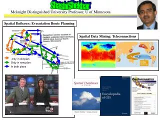
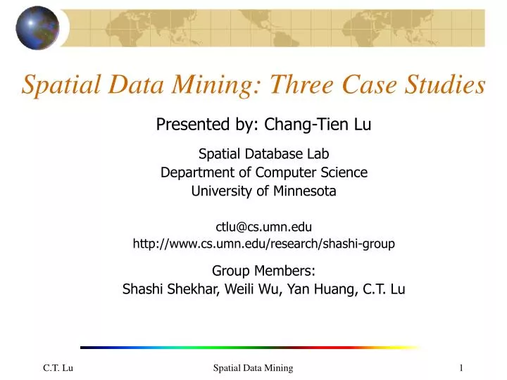
1. Spatial Data Mining: Three Case Studies Presented by: Chang-Tien Lu Spatial Database Lab Department of Computer Science University of Minnesota ctlu@cs.umn.edu http://www.cs.umn.edu/research/shashi-group Group Members: Shashi Shekhar, Weili Wu, Yan Huang, C.T. Lu Spatial Data Mining

2. Outline • Introduction • Case 1: Location Prediction • Case 2: Spatial Association: Co-location • Case 3: Spatial Outlier Detection • Conclusion and Future Directions Spatial Data Mining

3. Introduction: spatial data mining • Spatial Databases are too large to analyze manually • NASA Earth Observation System (EOS) • National Institute of Justice – Crime mapping • Census Bureau, Dept. of Commerce - Census Data • Spatial Data Mining • Discover frequent and interesting spatial patterns for post processing (knowledge discovery) • Pattern examples: spatial outliers, location prediction, clustering, spatial association, trends, .. • Historical Example • London, 1854 • Cholera & water pump Spatial Data Mining

4. Framework • Problem statement: capture special needs • Data exploration: maps • Try reusing classical methods • data mining, spatial statistics • Invent new methods if reuse is not applicable • Develop efficient algorithms • Validation, Performance tuning Spatial Data Mining

5. Case 1: Location Prediction • Problem: predict nesting site in marshes • Given vegetation, water depth, distance to edge, etc. • Data - maps of nests and attributes • spatially clustered nests, spatially smooth attributes • Classical method: logistic regression, decision trees, bayesian classifier • but, independence assumption is violated ! • Misses auto-correlation ! • Spatial auto-regression (SAR) • Open issues: spatial accuracy vs. classification accurary • Open issue: performance - SAR learning is slow! Spatial Data Mining

6. Location Prediction Given: 1.Spatial Framework 2. Explanatory functions: 3. A dependent class: 4. A family of function mappings: Find: Classification model: Objective:maximize classification_accuracy Constraints: Spatial Autocorrelation exists Nest locations Distance to open water Vegetation durability Water depth Spatial Data Mining

7. Evaluation: Change Model • Linear Regression • Spatial Autoregression Model (SAR) • y = Wy + X +  • W models neighborhood relationships •  models strength of spatial dependencies •  error vector • Mixed Spatial Autoregression Model (MSAR) • y = Wy + X + WX +  • Consider the impact of the explanatory variables from the neighboring observations Spatial Data Mining

8. Measure: ROC Curve • Classification accuracy: confusion matrix • ROC Curve: Locus of the pair (TPR,FPR) for each cut-off probability • Receiver Operating Characteristic (ROC) • TPR = AnPn / (AnPn + AnPnn) • FPR = AnnPn / (AnnPn+AnnPnn) Spatial Data Mining

9. Evaluation: Change Model • Linear Regression • Spatial Regression • Spatial model is better Spatial Data Mining

10. Solution Procedures • Spatial Autoregression Model (SAR) • y = Wy + X +  • Solutions •  and  - can be estimated using Maximum likelihood theory or Bayesian statistics. • e.g., spatial econometrics package uses Bayesian approach using sampling-based Markov Chain Monte Carlo (MCMC) method. • Maximum likelihood-based estimation requires O(n3) ops. Spatial Data Mining

11. Evaluation: Chang measure • Spatial accuracy (map similarity) • New measure: ADNP • Average distance to nearest prediction Spatial Data Mining

12. Predicting Location using Map Similarity Spatial Data Mining

13. Predicting location using Map Similarity • PLUMS components • Map Similarity : Avg. Distance to Nearest Prediction(ADNP) ,.. • Search Algorithm : Greedy, gradient descent • Function family : generalized linear (GL)(logit, probit), non-linear, • GL with auto-correlation • Discretization of parameter space : Uniform, non-uniform, • multi-resolution, … Spatial Data Mining

14. Association Rule • Supermarket shelf management • Goal: To identify items that are bought together by sufficiently many customers • Approach: Process the point-of-scale data collected with barcode scanners to find dependencies among items (Transaction data) • A classic rule – • If a customer buys diaper and milk, then he is very likely to buy beer • So, don’t be surprised if you find six-packs of beer stacked next to diapers! Spatial Data Mining

15. Association Rules:Support and confidence • Item set I = {i1, i2, ….ik} • Transactions T = {t1, t2, …tn} • Association rule: A -> B • Support S • (A and B) occur in at least S percent of the transactions • P (A U B) • Confidence C : • Of all the transactions in which A occurs, at least C percent of them contains B • P (B|A) Spatial Data Mining

16. Case 2: Spatial Association Rule • Problem: Given a set of boolean spatial features • find subsets of co-located features, • e.g. (fire, drought, vegetation) • Data - continuous space, partition not natural • Classical data mining approach: association rules • But, No Transactions!!! No support measure!! • Approach: Work with continuous data without transactionizing it! • Participation index (support) : min. fraction of instances of a features in join result • Confidence = Pr.[fire at s | drought in N(s) and vegetation in N(s)] • new algorithm using spatial joins Spatial Data Mining

17. Co-location Can you find co-location patterns from the following sample dataset? Answers: and Spatial Data Mining

18. Co-location Can you find co-location patterns from the following sample dataset? Spatial Data Mining

19. Co-location Spatial Co-location A set of features frequently co-located Given A set T of K boolean spatial feature types T={f1,f2, … , fk} A set P of N locations P={p1, …, pN } in a spatial frame work S, pi P is of some spatial feature in T A neighbor relation R over locations in S Find Tc = subsets of T frequently co-located Objective Correctness Completeness Efficiency Constraints R is symmetric and reflexive Monotonic prevalence measure Reference Feature Centric Window Centric Event Centric Spatial Data Mining

20. Co-location Comparison with association rules Participation index • Participation index = min{pr(fi, c)} • Participation ratio pr(fi, c) of feature fi in co-location c = {f1, f2, …, fk} • Fraction of instances of fi with feature {f1, f2, f i-1, f i+1,…, fk} nearby. Spatial Data Mining

21. Spatial Co-location Patterns • Dataset • Spatial feature A,B,C and their instances • Possible associations are (A, B), (B, C), etc. • Neighbor relationship includes following pairs: • A1, B1 • A2, B1 • A2, B2 • B1, C1 • B2, C2 Spatial Data Mining

22. Spatial Co-location Patterns • Partition approach [Yasuhiko, KDD 2001] • Support not well defined • i.e., not independent of execution trace • Has a fast heuristic which is hard to analyze for • correctness/completeness • Dataset Spatial feature A,B, C, and their instances Support (A,B) =2 (B,C)=2 Support (A,B)=1 (B,C)=2 Spatial Data Mining

23. Spatial Co-location Patterns • Reference feature approach [Han SSD 95] • Use C as reference feature to get transactions • Transactions: (B1) (B2) • Support (A,B) = Ǿ • Note: Neighbor relationship includes following • pairs: • A1, B1 • A2, B1 • A2, B2 • B1, C1 • B2, C2 • Dataset Spatial feature A,B, C, and their instances Spatial Data Mining

24. Spatial Co-location Patterns • Dataset • Our approach (Event Centric) • Neighborhood instead of transactions • Spatial join on neighbor relationship • Support • Participation index = Min ( p_ratio ) • P_ratio(A, (A,B)) = fraction of instance of A participating in join(A,B, neighbor) • Examples • Support(A, B)=min(3/2,3/2)=1.5 • Support(B, C)=min(2/2,2/2)=1 Spatial feature A,B, C, and their instances Spatial Data Mining

25. Spatial Co-location Patterns • Partition approach • Our approach • Dataset Support(A,B)=min(3/2,3/2)=1.5 Support(B,C)=min(2/2,2/2)=1 Support A,B =2 B,C=2 Spatial feature A,B, C, and their instances • Reference feature approach C as reference feature Transactions: (B1) (B2) Support (A,B) = Ǿ Support A,B=1 B,C=2 Spatial Data Mining

26. Case 3: Spatial Outliers Detection Spatial Outlier: A data point that is extreme relative to it neighbors Spatial Data Mining

27. Application Domain: Traffic Data Spatial Data Mining

28. Spatial Outlier Detection Given • A spatial framework SF consisting of locations s1, s2, …, sn • An attribute function f : si R (R : set of real numbers) • A neighborhood relationship N  SF  SF • A neighborhood aggregation function : RN R • A difference function Fdiff : R  R  R • Statistic test function ST : R { True, False } • Test is based on Fdiff (f, (f, N) Find O = {vi | vi V, vi is a spatial outlier} Objective Correctness: The attribute values of vi is extreme, compared with its neighbors Computational efficiency Spatial Data Mining

29. An example of Spatial outlier Spatial Data Mining

30. Spatial Outlier Detection: Zs(x) approach Function: If Declare x as a spatial outlier Spatial Data Mining

31. Evaluation of Statistical Assumption • Distribution of traffic station attribute f(x) looks normal • Distribution of looks normal too! Spatial Data Mining

32. Different Spatial Outlier Test • Spatial Statistic Approach • Scatter plot approach(Luc Anselin 94’) • Moran scatter plot approach (Luc Anselin 95’) • Variogram cloud approach (Graphic) Spatial Data Mining

33. Scatter plot approach • Given • An attribute function f(x) • A neighborhood relationship N(x) • An aggregation function • A difference function Fdiff: є = E(x) – (mf(x) + b) • Detect spatial outlier by • Statistic test function ST : Spatial Data Mining

34. Graphical Spatial Outlier Test Spatial Data Mining

35. Graphical Spatial Tests Original Data Spatial Data Mining

36. A Unified Algorithm • Separate two phases • Model building • Testing (a node or a set of nodes) • Computation structure of model building • Key insights: • Spatial self join using N(x) relationship • Algebraic aggregate functions can be computed in one disk scan of spatial join • Computation structure of testing • Single node: spatial range query • Get-All-Neighbors(x) operation Spatial Data Mining

37. An example: Scatter plot • Model building • An attribute function f(x) • Neighborhood aggregate function • Distributive aggregate functions • Algebraic aggregate functions • where , • Testing • Difference function • where • Statistic test function Spatial Data Mining

38. Outlier Stations Detected Spatial Data Mining

39. Outlier Station Detected Spatial Data Mining

40. Conclusion and Future Directions • Spatial domains may not satisfy assumptions of classical methods • data: auto-correlation, continuous geographic space • patterns: global vs. local, e.g., outliers vs. spatial outliers • data exploration: maps and albums • Open Issues • patterns: hot-spots, spatial trends,… • metrics: spatial accuracy (predicted locations), spatial contiguity(clusters) • spatio-temporal dataset: spatial-temporal outliers • scale and resolutions sentivity of patterns • geo-statistical confidence measure for mined patterns Spatial Data Mining

41. Reference • S. Shekhar and Y. Huang, “Discovering Spatial Co-location Patterns: a Summary of Results”, In Proc. of 7th International Symposium on Spatial and Temporal Databases (SSTD01), July 2001. • S. Shekhar, C.T. Lu, P. Zhang, "Detecting Graph-based Spatial Outliers: Algorithms and Applications“, the Seventh ACM SIGKDD International Conference on Knowledge Discovery and Data Mining, 2001. • S. Shekhar, C.T. Lu, P. Zhang, “Detecting Graph-based Saptial Outlier”, Intelligent Data Analysis, To appear in Vol. 6(3), 2002 • S. Chawla, S. Shekhar, W. Wu and U. Ozesmi, “Extending Data Mining for Spatial Applications: A Case Study in Predicting Nest Locations”, Proc. Int. Confi. on 2000 ACM SIGMOD Workshop on Research Issues in Data Mining and Knowledge Discovery (DMKD 2000), Dallas, TX, May 14, 2000. • S. Chawla, S. Shekhar, W. Wu and U. Ozesmi, “Modeling Spatial Dependencies for Mining Geospatial Data”, First SIAM International Conference on Data Mining, 2001. • S. Shekhar, Y. Huang, W. Wu, C.T. Lu, What's Spatial about Spatial Data Mining: Three Case Studies , as Chapter of Book: Data Mining for Scientific and Engineering Applications. V. Kumar, R. Grossman, C. Kamath, R. Namburu (eds.), Kluwer Academic Pub., 2001, ISBN 1-4020-0033-2 • Shashi Shekhar and Yan Huang , Multi-resolution Co-location Miner: a New Algorithm to Find Co-location Patterns in Spatial Datasets, Fifth Workshop on Mining Scientific Datasets (SIAM 2nd Data Mining Conference), April 2002 Spatial Data Mining

42. http://www.cs.umn.edu/research/shashi-group Thank you !!! Spatial Data Mining