Download
1 / 14
140 likes | 152 Views
7 The Mathematics of Networks. 7.1 Trees 7.2 Spanning Trees 7.3 Kruskal’s Algorithm 7.4 The Shortest Network Connecting Three Points 7.5 Shortest Networks for Four or More Points. Kruskal’s Algorithm.

E N D
7 The Mathematics of Networks 7.1 Trees 7.2 Spanning Trees 7.3 Kruskal’s Algorithm 7.4 The Shortest Network Connecting Three Points 7.5 Shortest Networks for Four or More Points
Kruskal’s Algorithm Kruskal’s algorithm is almost identical to the cheapest-linkalgorithm: We build the minimum spanning tree one edgeat a time, choosing at each step the cheapest available edge. The only restriction toour choice of edges is that we should never choose an edge that creates a circuit.(Having three or more edges coming out of a vertex, however, is now OK.) Whatis truly remarkable about Kruskal’s algorithm is that–unlike the cheapest-link algorithm–it always gives an optimal solution.
Example 7.7 The Amazonian Cable Network: Part 2 What is the optimal fiber-opticcable network connecting the seven towns shown?
Example 7.7 The Amazonian Cable Network: Part 2 The weightedgraph shows the costs (in millions of dollars) of laying the cablelines along each of the potential links of the network.
Example 7.7 The Amazonian Cable Network: Part 2 The answer, as we now know, is to find the MST of the graph. We will use Kruskal’s algorithm to do it. Here are the details:
Example 7.7 The Amazonian Cable Network: Part 2 Step 1.Among all the possible links, we choose the cheapest one, in this particular case GF (at a cost of $42 million). This link is going to be part of the MST,and we mark it in red (or any other color) as shown
Example 7.7 The Amazonian Cable Network: Part 2 Step 2.The next cheapest link available is BD at $45 million. We choose it forthe MST and mark it in red. Step 3.The next cheapest link available is AD at $49 million. Again, wechoose it for the MST and mark it in red.
Example 7.7 The Amazonian Cable Network: Part 2 Step 4.For the next cheapest link there is a tie between AB and DG, both at$51 million. But we can rule out AB–it would create a circuit in the MST,and we can’t have that! The link DG, on the other hand, is just fine, so we markit in red and make it part of the MST.
Example 7.7 The Amazonian Cable Network: Part 2 Step 5.The next cheapest link available is CD at $53 million. No problemshere,so again, we mark it in red and make it part of the MST. Step 6.The next cheapest link available is BC at $55 million, but this linkwould create a circuit, so we cross it out. The next possible choice is CF at $56million, but once again, this choice creates a circuit so we must cross it out.The next possible choice is CE at $59 million, and this is one we do choose.We mark it in red and make it part of the MST.
Example 7.7 The Amazonian Cable Network: Part 2 Step ...Wait a second–we are finished! Even without looking at a picture,we can tell we are done–six links is exactly what is needed for an MST onseven vertices. The figure shows the MST in red. The total cost of the network is$299 million.
KRUSKAL’S ALGORITHM Step 1 Pick the cheapest link available. (In case of a tie, pick one at random.)Mark it (say in red). Step 2.Pick the next cheapest link available and mark it. Steps 3, 4, ..., N–1.Continue picking and marking the cheapest unmarkedlink available that does not create a circuit.
Kruskal’s Algorithm As algorithms go, Kruskal’s algorithm is as good as it gets. First, it is easy toimplement. Second, it is an efficient algorithm. As we increase the number of vertices and edges of the network, the amount of work grows more or less proportionally (roughly speaking, if finding the MST of a 30-city network takes you, say,30 minutes, finding the MST of a 60-city network might take you 60 minutes).
Kruskal’s Algorithm Last, but not least, Kruskal’s algorithm is an optimalalgorithm–it will alwaysfind a minimum spanning tree.Thus, we have reached a surprisingly satisfying end to the MST story: Nomatter how complicated the network, we can find its minimum spanning tree bymeans of an algorithm that is easy to understand and implement, is efficient, andis also optimal.