Download
1 / 58
680 likes | 980 Views
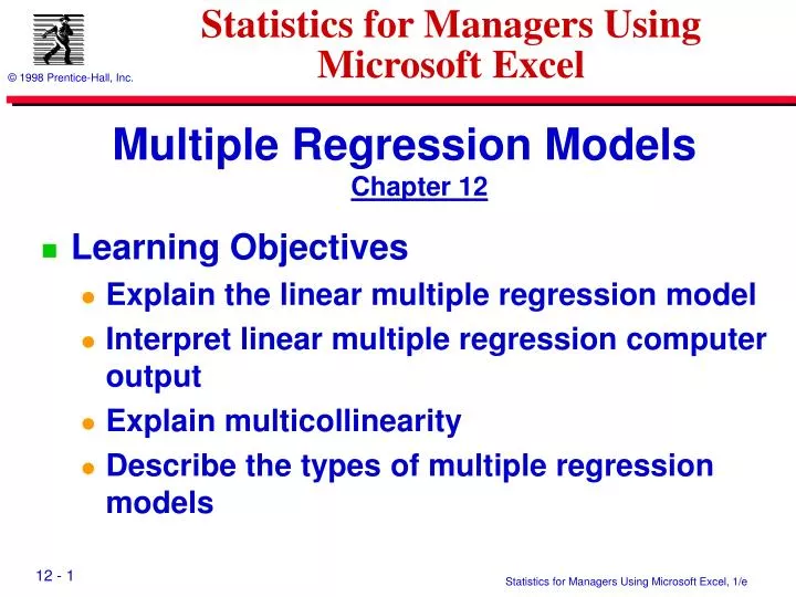
Statistics for Managers Using Microsoft Excel. Multiple Regression Models Chapter 12 Learning Objectives Explain the linear multiple regression model Interpret linear multiple regression computer output Explain multicollinearity Describe the types of multiple regression models.

E N D
Statistics for Managers Using Microsoft Excel Multiple Regression ModelsChapter 12 • Learning Objectives • Explain the linear multiple regression model • Interpret linear multiple regression computer output • Explain multicollinearity • Describe the types of multiple regression models
Linear Multiple RegressionModel • Relationship between 1 dependent & 2 or more independent variables is a linear function Population Y-intercept Population slopes Random error Dependent (response) variable Independent (explanatory) variables
PopulationMultiple RegressionModel Bivariate model
Sample Multiple RegressionModel Bivariate model
Regression Modeling Steps • Define problem or question • Specify model • Collect data • Do descriptive data analysis • Estimate unknown parameters • Evaluate model • Use model for prediction
Multiple Linear Regression Equations Too complicated by hand! Ouch!
Interpretation of Estimated Coefficients • Slope (bP) • Estimated Y changes by bP for each 1 unit increase in XPholding all other variables constant • Example: If b1 = 2, then Sales (Y) is expected to increase by 2 for each 1 unit increase in Advertising (X1) given the Number of Sales Rep’s (X2) • Y-Intercept (b0) • Average value of Y when XP = 0
Parameter Estimation Example You work in advertising for the New York Times. You want to find the effect of ad size (sq. in.) & newspaper circulation (000) on the number of ad responses (00). You’ve collected the following data: RespSizeCirc 1 1 2 4 8 8 1 3 1 3 5 7 2 6 4 4 10 6
ParameterEstimation Excel Output bP b0 b2 b1
Interpretation of Coefficients Solution • Slope (b1) • # Responses to Ad is expected to increase by .2049 (20.49) for each 1 sq. in. increase in Ad Size holding Circulation constant • Slope (b2) • # Responses to Ad is expected to increase by .2805 (28.05) for each 1 unit (1,000) increase in Circulationholding Ad Size constant
Regression Modeling Steps Evaluating Multiple Regression Model Steps • Define problem or question • Specify model • Collect data • Do descriptive data analysis • Estimate unknown parameters • Evaluate model • Use model for prediction
Evaluating Multiple Regression Model Steps • Examine variation measures • Do residual analysis • Test parameter significance • Overall model • Portions of model • Individual coefficients • Test for multicollinearity
Evaluating Multiple Regression Model Steps • Examine variation measures • Do residual analysis • Test parameter significance • Overall model • Portions of model • Individual coefficients • Test for multicollinearity Expanded! New! New! New!
Coefficient of Multiple Determination • Proportion of variation in Y ‘explained’ by all X variables taken together • r2Y.12..P = Explained variation = SSR Total variation SST • Never decreases when new X variable is added to model • Only Y values determine SST • Disadvantage when comparing models
Adjusted Coefficient of Multiple Determination • Proportion of variation in Y ‘explained’ by all X variables taken together • Reflects • Sample size • Number of independent variables • Smaller than r2Y.12..P • Used to compare models
Evaluating Multiple Regression Model Steps • Examine variation measures • Do residual analysis • Test parameter significance • Overall model • Portions of model • Individual coefficients • Test for multicollinearity Expanded! New! New! New!
Testing Overall Significance • Shows if there is a linear relationship between all X variables together & Y • Uses F test statistic • Hypotheses • H0: 1 = 2 = ... = P = 0 • No linear relationship • H1: At least one coefficient is not 0 • At least one X variable affects Y
Evaluating Multiple Regression Model Steps • Examine variation measures • Do residual analysis • Test parameter significance • Overall model • Portions of model • Individual coefficients • Test for multicollinearity Expanded! New! New! New!
Multicollinearity • High correlation between X variables • Coefficients measure combined effect • Leads to unstable coefficients depending on X variables in model • Always exists; matter of degree • Example: Using both Sales & Profit as explanatory variables in same model
Detecting Multicollinearity • Examine correlation matrix • Correlations between pairs of X variables are more than with Y variable • Examine variance inflation factor (VIF) • If VIFj > 5, multicollinearity exists • Few remedies • Obtain new sample data • Eliminate one correlated X variable
Polynomial (Curvilinear) Regression Model • Relationship between 1 dependent & 2 or more independent variables is a quadratic function • Useful 1st model if non-linear relationship suspected
Polynomial (Curvilinear) Regression Model • Relationship between 1 dependent & 2 or more independent variables is a quadratic function • Useful 1st model if non-linear relationship suspected • Polynomial model Curvilinear effect Linear effect
Polynomial (Curvilinear) Model Relationships 11 > 0 11 > 0 11 < 0 11 < 0
Polynomial (Curvilinear) Model Worksheet Create X12 column. Run regression with Y, X1, X12
Dummy-Variable Regression Model • Involves categorical X variable with 2 levels • e.g., male-female, college-no college etc. • Variable levels coded 0 & 1 • Assumes only intercept is different • Slopes are constant across categories
Dummy-Variable Regression Model • Involves categorical X variable with 2 levels • e.g., male-female, college-no college etc. • Variable levels coded 0 & 1 • Assumes only intercept is different • Slopes are constant across categories • Dummy-variable model
Dummy-Variable Model Worksheet X2 levels: 0 = Group 1; 1 = Group 2. Run regression with Y, X1, X2
Interpreting Dummy-Variable Model Equation Y b b X b X Given: i 0 1 1 i 2 2 i Y Starting s alary of c ollege gra d' s X GPA 1 { 0 i f Male X 2 1 if Female
Interpreting Dummy-Variable Model Equation Y b b X b X Given: i 0 1 1 i 2 2 i Y Starting s alary of c ollege gra d' s X GPA 1 { 0 i f Male X 2 1 if Female Males ( X 0 ): 2 (0) Y b b X b b b X i 0 1 1 i 2 0 1 1 i
Interpreting Dummy-Variable Model Equation Y b b X b X Given: i 0 1 1 i 2 2 i Y Starting s alary of c ollege gra d' s X GPA 1 { 0 i f Male X 2 1 if Female Same slopes Males ( X 0 ): 2 (0) Y b b X b b b X i 0 1 1 2 0 1 1 Females (X2 = 1): b (1) Y b b X b b X b 2 1 1 2 1 1 i 0 0
Dummy-Variable Model Relationships Y Same slopes b1 Females b0 + b2 b0 Males 0 X1 0
Dummy-Variable Model Example Y 3 5 X 7 X Computer O utput: i 1 i 2 i { 0 i f Male X 2 1 if Female
Dummy-Variable Model Example Y 3 5 X 7 X Computer O utput: i 1 i 2 i { 0 i f Male X 2 1 if Female Males ( X 0 ): 2 Y 3 5 X 7 3 5 X (0) i 1 i 1 i
Dummy-Variable Model Example Y 3 5 X 7 X Computer O utput: i 1 i 2 i { 0 i f Male X 2 1 if Female Same slopes Males ( X 0 ): 2 Y 3 5 X 7 3 5 X (0) i 1 i 1 i Females ( X 1 ): 2 10 X X Y 3 5 5 (1) 7 i i i 1 1
Interaction Regression Model • Hypothesizes interaction between pairs of X variables • Response to one X variable varies at different levels of another X variable
Interaction Regression Model • Hypothesizes interaction between pairs of X variables • Response to one X variable varies at different levels of another X variable • Contains two-way cross product terms
Interaction Regression Model • Hypothesizes interaction between pairs of X variables • Response to one X variable varies at different levels of another X variable • Contains two-way cross product terms • Can be combined with other models • e.g., dummy variable model
Effect of Interaction • Given:
Effect of Interaction • Given: • Without interaction term, effect of X1 on Y is measured by 1
Effect of Interaction • Given: • Without interaction term, effect of X1 on Y is measured by 1 • With interaction term, effect of X1 onY is measured by 1 + 3X2 • Effect increases as X2i increases
Interaction Example Y = 1 + 2X1 + 3X2 + 4X1X2 Y 12 8 4 0 X1 0 0.5 1 1.5
Interaction Example Y = 1 + 2X1 + 3X2 + 4X1X2 Y 12 8 Y = 1 + 2X1 + 3(0) + 4X1(0) = 1 + 2X1 4 0 X1 0 0.5 1 1.5
Interaction Example Y = 1 + 2X1 + 3X2 + 4X1X2 Y Y = 1 + 2X1 + 3(1) + 4X1(1) = 4 + 6X1 12 8 Y = 1 + 2X1 + 3(0) + 4X1(0) = 1 + 2X1 4 0 X1 0 0.5 1 1.5
Interaction Example Y = 1 + 2X1 + 3X2 + 4X1X2 Y Y = 1 + 2X1 + 3(1) + 4X1(1) = 4 + 6X1 12 8 Y = 1 + 2X1 + 3(0) + 4X1(0) = 1 + 2X1 4 0 X1 0 0.5 1 1.5 Effect (slope) of X1 on Y does depend on X2 value
Interaction Regression Model Worksheet Multiply X1by X2 to get X1X2. Run regression with Y, X1, X2 , X1X2