Download
1 / 62
660 likes | 918 Views
Reversible Logic Synthesis with Garbage Bits. Lecture 6. Marek Perkowski. Logic Synthesis for Quantum Pseudo-Binary Logic (Permutation Logic). Background. Reviev of Reversible logic. This approach is mostly for quantum logic realization.

E N D
Reversible Logic Synthesis with Garbage Bits Lecture 6 Marek Perkowski
Logic Synthesis for Quantum Pseudo-Binary Logic (Permutation Logic)
Background Reviev of Reversible logic This approach is mostly for quantum logic realization For optical and CMOS realizations the k*k assumption is not necessarily used
Q R C AC’+B BC’+AC P 0 1 B C Q R P 0 1 0 1 A C A B C A A circuit from two multiplexers B Its schemata This is a reversible gate, one of many Notation for Fredkin Gates
Margolus Gate Q R P 0 1 0 1 0 1 A A B C C A B Reversible Conservative 3*3 gate There are many similar gates
Toffoli Gate P Q R • The 3 * 3 Toffoli gate is described by these equations: P = A, Q = B, R = AB C, • Toffoli gate is an example of two-through gates, because two of its inputs are given to the output. + * A B C
Feynman, Toffoli and Fredkin gates are their own inverses P Q R P Q + + * A B C A B Feynman (b) Toffoli P Q R + + 1 0 * * C A B Kerntopf Gate
Kerntopf Gate • The Kerntopf gate is described by equations: P = 1 A B C AB, Q = 1 AB B C BC, R = 1 A B AC. • When C=1 then P = A + B, Q = A * B, R = B, so AND/OR gate is realized on outputs P and Q with C as the controlling input value. • When C = 0 then P = A * B, Q = A + B, R = A B. • 18 different cofactors! Review cofactors if students forgot
Kerntopf Gate • As we see, the 3*3 Kerntopf gate is not a one-through nor a two-through gate. • Despite theoretical advantages of Kerntopf gate over classical Fredkin and Toffoli gates, so far there are no published results on realization of this gate. • Is it better for no-ancilla synthesis?
Feynman Feynman How to build garbage-less circuits D F1 Fredkin GARBAGE BIT 1 A Toffoli B C GARBAGE BIT 2 2 outputs 2 garbages width = 4 delay = 4 F2 We can decrease garbage at the cost of delay and number of gates We create inverse circuit and add spies for all outputs
Fredkin D Feynman A Toffoli B C Feynman copy copy How to build garbage-less circuits Feynman D Fredkin A Toffoli B C Feynman inputs reconstructed F1 from spy F2 from spy 2 outputs no garbage width = 4 delay = 9 A,B,C,D are original inputs This process is informationally reversible It can be in addition thermodynamically reversible
Observations • We reduced garbage at the cost of delay and number of gates • We were not able to reduce the width of the scratchpad register
Goals of reversible logic synthesis 1. Minimize the garbage 2. Minimize the width of scratchpad register 3. Minimize the total number of gates 4. Minimize the delay
Preprocessing Synthesis from (p)KFDDs
+ + + + * * * * Previous levels f4 f1 f2 f3 …... Other same level …... ci …... k4 k2 k1 k3 k5 k6 next levels
+ + + + * * * * Previous levels f4 f1 f2 f3 …... Other same level …... ci …... k4 k2 k1 k3 k5 k6 next levels
Example of converting a decision diagram to reversible circuit
f g + + d * * S pD S nD S S S d 1 1 d a 1 0 0 a 1 1 0 0 1 b c e 1 0 g G1 G2 f (a) d e (b) G3 0 1 0 1 0 1 c b
S S S S S S S S S S y1 1 0 x4 1 0 y2 x1 0 1 0 1 0 1 y3 0 1 x3 1 0 0 1 1 0 1 0 x2 0 1 0 1 (a) (b) • y1 =x2 x3 x1x3 • y2 =x3 x1 x1x4 • y3 =x1 x4 x3x4 • y4 =x4 Nonlinear preprocessor Corresponding fDD of Kerntopf Standard BDD Converting fDDs to reversible circuits
x3 • y1 =x2 x3 x1x3 • y2 =x3 x1 x1x4 • y3 =x1 x4 x3x4 • y4 =x4 * x1 y1 x2 + h G1 x1 * x4 1 0 0 1 y2 + G3 * G2 x4 y3 + x3 Reversible circuit corresponding to fDD together with preprocessor 1 + x3
Open Problems: • Is our set of mapping rules sufficient? • (we have currently about 20 rules, but many more can be created). • What is the practically best starting point for large functions? KFDD? PKFDD? fDD? • How to transform the diagram or the circuit to improve the cost function? • What to do in case of rule conflict? • How to create rules to decrease garbage?
Use of Reversibility Observation: Every synthesis method can be executed forward and backwards Sometimes solution backwards can be simpler
Function F Function F -1 A B C D 0 0 0 0 0 0 0 1 0 0 1 0 0 0 1 1 0 1 0 0 0 1 0 1 0 1 1 0 0 1 1 1 1 0 0 0 1 0 0 1 1 0 1 0 1 0 1 1 1 1 0 0 1 1 0 1 1 1 1 0 1 1 1 1 X Y Z V 0 0 1 1 1 0 1 1 0 0 1 0 1 0 1 0 0 0 0 0 0 1 1 1 0 0 0 1 0 1 1 0 1 1 1 1 1 0 0 0 1 1 1 0 1 0 0 1 1 1 0 1 0 1 0 1 1 1 0 0 0 1 0 0 A B C D 0 1 0 0 0 1 1 0 0 0 1 0 0 0 0 0 1 1 1 1 1 1 0 1 0 1 1 1 0 1 0 1 1 0 0 1 1 0 1 1 0 0 1 1 0 0 0 1 1 1 1 0 1 1 0 0 1 0 1 0 1 0 0 0 X Y Z V 0 0 0 0 0 0 0 1 0 0 1 0 0 0 1 1 0 1 0 0 0 1 0 1 0 1 1 0 0 1 1 1 1 0 0 0 1 0 0 1 1 0 1 0 1 0 1 1 1 1 0 0 1 1 0 1 1 1 1 0 1 1 1 1 Several methods exist to calculate inverse from forward function Forward Function Inverse Function
Feynman Feynman Feynman Feynman D Y Fredkin A Toffoli B C Z V Circuit for function F X F*F-1=I D Y Fredkin X Circuit for function F -1 A Toffoli B C Z V
Method of realization of F • 1. Find function inverse F-1 of function F. • 2. Synthesize F-1 using any method for reversible gates • 3. Draw the schematics of F-1 from gates. • 4. In the schematics replace every gate by its reverse and change the direction of signals. • 5. The new schematics is the realization of F.
Feynman Feynman Feynman Feynman Feynman X X D Y Y Y X=G1 Y Fredkin A YZ Fredkin 0 Y+Z B YZ Fan-out gate G2=ZV 0 YZ Z Fan-out gate C =ZV YZ Another realization of F-1 Z ZV We were not able to find the best realization of F-1 shown earlier V
Composition Methods • Composition methods with matching-based cell selection and complexity measures have been presented by: • Dietmeyer • Schneider • Wojcik • Michalski • Jozwiak, Chojnacki and Volf • DeMicheli library matching • Kravets and Sakallah
Uses library of 1*1,2*2 and 3*3 cells For every 3*3 function, a ready solution cascade is stored - see the results of Kerntopf and Storme-DeVos For every reversible gate, all cofactors can be stored (constants and garbage) and used in NPN matching. Gates with more cofactors (like Kerntopf) are better
Uses equivalence mapping transformations based on NPN-equivalence Synthesis from inputs to outputs and from outputs to inputs, backtracking and look-ahead strategies All intermediate functions calculated in terms of input variables Can be applied to both classical reversible and quantum logic
How to select the cell, its alignment and constants? • Select the gate that provides smallest complexity evaluation of the remaining functions and intermediate functions. • This works for both forward and backward transformations • I proposed PPRM for matching because it is easy to implement. Other representations and measures can be used for matching - De Micheli, Dietmeyer, Jozwiak. • Solve exor equations to find inverse functions and input values. Sometimes Kmaps are easier to use.
Direction of synthesis a a x c 0 c ab s 1 b y + b t + 0 cab 1 a a First stage of decomposition: Feynman gate Third stage of decomposition: Feynman gate Second stage of decomposition: Fredkin gate Decompositional synthesis of Toffoli Gate from Fredkin and Feynman Gates Using PPRM representation allows for NPN matching and good evaluation of the remaining function complexity
Direction of synthesis a a x c 0 c ab s 1 b y + t b + 0 cab 1 a a Third stage of composition: Feynman gate First stage of composition: Feynman gate Second stage of composition: Reversible Expansion for Fredkin gate Compositional synthesis of Toffoli Gate from Fredkin and Feynman Gates NPN matching takes care of permutations and inverters
CompositionFrom inputs to outputs What to do if the initial function is not reversible?
Composition Restrict to C=0 Toffoli 3. Toffoli gate assumed. 4. New functions X,Y,Z created. 5. C=0 restriction taken 6. Functions h and g of X,Y,Z can be now realized A B C 0 0 0 0 0 1 0 1 0 0 1 1 1 0 0 1 0 1 1 1 0 1 1 1 X Y Z 0 0 0 0 0 1 0 1 0 0 1 1 1 0 0 1 0 1 1 1 1 1 1 0 h=AB g=A*BG 0 0 - 0 0 - 1 0 - 1 0 - 1 0 - 1 0 - 0 1 - 0 1 - 2. These are outputs 1. These are inputs Z=A*B
Feynman garbage G =X=A X=A A h=XY=AB Y=B Toffoli B Z=AB g=Z=AB C =0 IDEA: Look to outputs, modify near inputs, reduce the difference Created first Calculated in terms of new variables X,Y,Z and selected Feynman gate Compositional synthesis of non-reversible function of half-adder
Adder is composed from half-adders Compositional synthesis is here top-down, hierachical, like in classical CMOS 2 garbage bits and one constant
G =X=A X=A A Feynman h=XY=AB Y=B Toffoli B Z=AB g=Z=AB C =0 Another variant assumes Kerntopf gate
A A CN B CCN A B (Sum) 0 A and B (Carry) Feynman Toffoli Heuristics for finding simplest reversible function during composition A B A B A B A * B AB 0 Mapping of a half-adder AB 00 01 11 10 001001 10 This is what we would like to have But this is not reversible,
Heuristics for finding simplest reversible function during composition A A CN B CCN A B (Sum) AB 00 01 11 10 0 A and B (Carry) 001001 10 Feynman Toffoli A B A B A B A * B AB 0 Mapping of a half-adder The simplest way to separate them is to add variable A
Heuristics for finding simplest reversible function during composition A A B A B A A CN B CCN A B (Sum) 0 A and B (Carry) Feynman Toffoli A B A * B AB 0 Mapping of a half-adder AB 00 01 11 10 000010101110 But this is not reversible, because more outputs than inputs This is what we would like to have
Heuristics for finding simplest reversible function during composition A B C A A B A A CN B CCN A B (Sum) 0 A and B (Carry) Feynman Toffoli A B A * B C AB 0 Mapping of a half-adder AB C 000010101110 Now function is reversible of A,B,C arguments. But we still need to decompose it to known gates 001011100111 Positive Davio Gate
Search • Search is defined by: • selecting function to be realized • selecting a gate type • selecting its forward or backwards matching • selecting other signals to match • selecting constant Garbage functions are becoming less and less undefined in the process of decomposition They can be used for synthesis • We adopt classical AI search algorithms • (depth-first, breadth-first, A*,best bound, etc)
Search • Search cannot be avoided • Trade-off between quality of solution and search time • The only real improvement is possible through better selection heuristics and better implementation of cell library.
P + * + forward backward Illustration of cooperation of various methods to design the Kerntopf gate from Fredkin, Toffoli, Feynman gates and inverters. One fan-out gate for input a, inverter for c and two fan-out gates for c are not shown. start g1 = ab + bc H= c+b Q G2 = b + c G3 0 1 0 1 0 1 0 1 R b c a c 1 forward G4 a c Library matching
... H G ... ... ... H H G ... G ... Curtis-like Ashenhurst-like New Curtis parallel serial