Download
1 / 18
180 likes | 588 Views
By: Chris Markson Student Adviser: Dr. Kaufman. Implementing the Probability Matrix Technique for Positron Emission Tomography. Introduction. PET vs. CAT PET ~ metabolic CAT ~ anatomical The Process Tagged chemical compound Positrons in compound meet electrons in the body~ annihilation

E N D
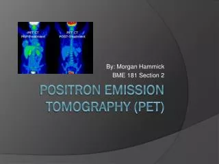
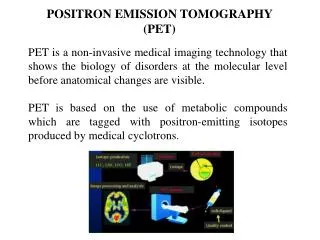
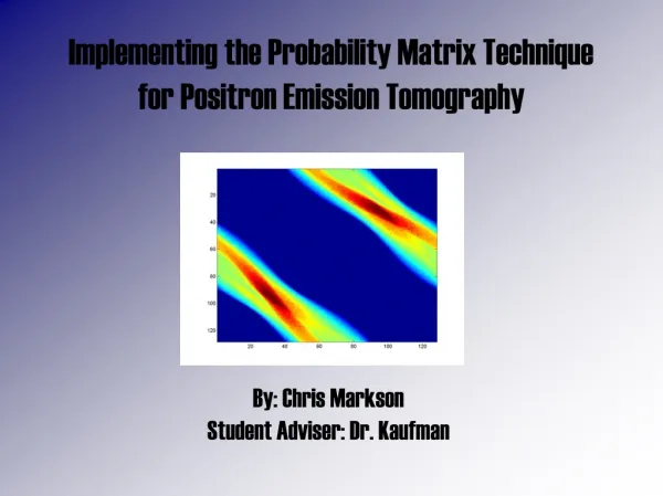
By: Chris Markson Student Adviser: Dr. Kaufman Implementing the Probability Matrix Technique for Positron Emission Tomography
Introduction • PET vs. CAT • PET ~ metabolic • CAT ~ anatomical • The Process • Tagged chemical compound • Positrons in compound meet electrons in the body~ annihilation • Photons produced at 180° • Detection • Problem: Reconstruct the image using the tube data
Grids • Put grid over organ of interest • 2 dimensions - pixels • 3 dimensions - voxels • Finer grid, more detail • Finer grid, more computation time and space
Probability Matrix Approach • C(tubes,pixels) = probability that events in a pixel will be detected by a tube • If 128 detectors, 128 pixels on a side,125 million elements • About 1% nonzero • Want to find the emissions x to approximate tube data y such that C x ~ y and x>=0 • Sum of the elements in x should equal the sum of the elements in y so all annihilations are accounted for • Use iterative approaches that only require matrix vector multiplication
My Responsibilities • Translate from FORTRAN into C++ and speed up code that generates the C matrix and does matrix by vector multiplication • Take out redundant code for successive subroutine calls • FORTRAN was very unstructured • Because have more memory, do not have to use circular symmetry – does this lead to faster code? • If one uses structures and linked lists – does this help? • Prior research suggested that EM algorithm for maximum likelihood works better from uniform starting guess rather than random • Does starting with solution from coarser grid help? • Should you smooth coarser grid solution?
EM Algorithm • One iteration: • Set s = CTx • Set z = y(t)/st for t = 1, 2, . . . , T. • Set w = Cz • Set xbnew = xbwb for b = 1, 2, . . . , B.
Image Output • Images Studied • 10 million vs. 1 million probabilities • Uniform guess – total tube count divided by number of pixels • Block expansion • Start with 64x64 data, EM Algorithm, expand to 128x128(1 pixel becomes 4 pixels), old solution becomes initial guess for 2nd EM run • Smoothed expansion • Same procedure, (1 pixel becomes 4 pixels) averaging middle pixels after expansion • Best image produced with tumors standing out
Tube Data 128x128 ~ 1m 64x64 ~ 1m smoothed 128x128 ~ 10m
block10m64x64 initial guess into EM, block expansion. uniform10mNo expansion, uniform initial guess. wexpand10m64x64 initial guess into EM, smoothed expansion.**Best result**
block1m64x64 initial guess into EM, block expansion. uniform1mNo expansion, uniform initial guess. wexpand1m64x64 initial guess into EM, smoothed expansion.
smuniform1mSmoothed first. No expansion, uniform initial guess. smwblockexpand1mSmoothed first. 64x64 initial guess into EM, block expansion. smwexpand1mSmoothed first. 64x64 initial guess into EM, smoothed expansion.
diffexbl1mDifference between smoothed expansion and block expansion smdiffexbl1mSmoothed tube data. Difference between smoothed expansion and block expansion smdiffunex1mSmoothed tube data. Difference between uniform and smoothed expansion.
Removal of repeating triangle code • Entire code much slower when compared to the repeating triangle code • EM algorithm faster • Removal of encode, decode, a1, a2 functions. Easier matrix by vector multiplication • Creating C matrix takes longer Full Square Code
Times All timings performed on Intel 1.4 GHz Centrino Chip, 512 MB RAM
Linked List • Theory: Having pointers to first element in each array save on offset calculations used in arrays. • EM() (16 iterations) • No LL • Avg processing time: 1214.7ms • With LL • Avg processing time: 6906.7ms • Difference: With LL 5692.0msslower
Linked List Times (continued) • Program Times: • No LL: • Avg processing time: 4743.0ms • With LL • Avg processing time: 12778.0ms • Difference: With LL 8035.0msslower
Tools Used • Original Code ~ FORTRAN • Translated and manipulated ~ C++ • Image manipulation and analysis ~ MATLAB