Download
1 / 29
290 likes | 427 Views
Topic 6 - Image Filtering - I. Department of Physics and Astronomy. DIGITAL IMAGE PROCESSING Course 3624. Professor Bob Warwick. 6. Image Filtering I: Spatial Domain Filtering.

E N D
Topic 6 - Image Filtering - I Department of Physics and Astronomy DIGITAL IMAGE PROCESSING Course 3624 Professor Bob Warwick
6. Image Filtering I: Spatial Domain Filtering The goal of spatial filtering is typically either to (a) reduce the impact of noise in the image via image smoothing or (b) to sharpen the detail within the image. Both processes involve the suppression and/or enhancement of particular spatial frequency components in the image (see Topic 8). Neighbourhood process (eg. Spatial filtering) Point process (eg. Mapping) • Procedure • Define an array of values known variously as the mask, filter, operator etc.. (usually with a 3 x 3 or 5 x 5 or 7 x 7 etc.. format) (ii) Compute a new image gxy from the old image fxy via: For a mask of dimension n x n (n odd), where m = (n-1)/2 is the central element. Calculate for all x & y Note that the denominator is a normalisation factor – sometimes not applicable!
Computing the 2-d Result original 3x3 average
6.1 Smoothing Filters • Smoothing filters involve calculating the average value (with some defined weighting) within the masked region. • Assuming a 3 x 3 format, some possibilities are: • 1 1 1 Replaces the original value with • 1 1 1 the average of 9 values (the central • 1 1 pixel plus its 8 nearest neighbours) • 1 1 1 Double weighting of the central pixel • 1 2 1 • 1 1 • 0 1 0 Replaces the original value with • 1 1 the average of 5 values (the central • 0 1 0 pixel plus its 4 nearest neighbours)
Smoothing Examples: Original Images Author: Richard Alan Peters II
Image Smoothing Examples Original Smoothed
Calculating the effective noise reduction Gaussian Distribution P(f) mean and standard deviation f Example Applying a 3 x 3 smoothing filter with unit coefficients results in a factor 3 reduction in the noise.
133 133 140 147 152 154 163 164 171 The Median Filter Smoothing filters can be used to reduce the impact of the noise in an image but also cause unwanted blurring. The larger the dimension of the smoothing mask the greater the noise reduction factor but also the greater the blurring. Non-linear filters, such as the Median Filter, can to some degree “decouple” these two effects – but in a way which is hard to quantify. The median filter would replace the central value with the median value contained within the mask (or window) region.
Suppression of Impulsive Noise Median Filter Smoothing Filter
The objective is to enhance the detail in the image by accentuating edges and boundaries. 6.2 Sharpening Filters Smoothing Averaging Sharpening Differencing In practice with discrete variables differencing is equivalent to differentiation and both the 1st and 2nd differentials can be used to mark the position in an image where there are rapid changes in gray level (ie edges). Continuous variables
Types of Filters Used in Image Sharpening - I Pairs of masks of various formats which give the vertical (axy) and horizontal (bxy) gradients: (i) The Roberts Operators (ii) (iii) The Prewitt Operators Where the final gradient image is calculated as:
Image Sharpening Examples … 0 0 0 0 1 1 1 ….. … 0 0 0 0 1 1 1 ….. … 0 0 0 0 1 1 1 ….. … 0 0 0 0 1 1 1 ….. Consider an image consisting of: Applying the following filters gives: (i) (ii) … 0 0 0 0 0 0 0 ….. … 0 0 0 0 0 0 0 ….. … 0 0 0 0 0 0 0 ….. … 0 0 0 0 0 0 0 ….. … 0 0 0 3 3 0 0 ….. … 0 0 0 3 3 0 0 ….. … 0 0 0 3 3 0 0 ….. … 0 0 0 3 3 0 0 …..
Calculating the Gradient Image The Sobel Operators
Types of Filters Used in Image Sharpening - II Masks which give the 2nd differential or Laplacian image (i) (ii) (iii)
255 510 -1 -1 0 -1 4 -1 -1 2 -1 2 -255 -1 -1 The 1-d and 2-d Laplacian Mask in Action
The Image Sharpening Process In image sharpening the usual approach is to add the derived ‘gradient’ or ‘Laplacian’ image to the original image in a process known as high frequency emphasis. Thus: Final image = original image + gradient or Laplacian image For the Laplacian case this can be achieved in one step by modifying the 2-d mask to: or
Image Sharpening Examples … 0 0 0 0 1 1 1 ….. … 0 0 0 0 1 1 1 ….. … 0 0 0 0 1 1 1 ….. … 0 0 0 0 1 1 1 ….. Consider an image consisting of: Applying the following filters gives: (i) (ii) … 0 0 0 -3 3 0 0 ….. … 0 0 0 -3 3 0 0 ….. … 0 0 0 -3 3 0 0 ….. … 0 0 0 -3 3 0 0 ….. … 0 0 0 -3 4 1 1 ….. … 0 0 0 -3 4 1 1 ….. … 0 0 0 -3 4 1 1 ….. … 0 0 0 -3 4 1 1 …..
The Mathematical Process of Spatial Filtering Consider the 1-d case of spatial filtering with an n element mask (n odd), where m= (n-1)/2 and ignoring the normalization factor. x i i' i'' a Equation 4 is the discrete version of the CONVOLUTION INTEGRAL. SPATIAL FILTERING IS A CONVOLUTION PROCESS
Practical Considerations • Edge Errors • For an n x n mask there is a (n-1)/2 border to the new image where exact values cannot be calculated. Solutions are: • Reduce the dimensions of the new image (usually impractical) • Calculate approximate values for the border pixels • Compute the cyclic convolution (beyond our scope). • Separability • A 2-d mask is separable if the successive application of two 1-d masks gives the equivalent result to the application of the 2-d mask. • For example, considered as matrices: • Therefore this smoothing mask is separable. • There are computational advantages if the mask is separable. Note: Both gradient and Laplacian filters can also be used in EDGE DETECTION – see topic 10