Download
1 / 29
290 likes | 491 Views
Repeats, Pseudogenes etc. Lecture 11/4. Paper : Wexler et al. Finding Approximate Tandem Repeats in Genomic Sequences Recomb 2004. Goal. Find approximate tandem repeat (ATR) A string of bases repeated consecutively at least twice with small differences between instances. ATR hunter.

E N D
Repeats, Pseudogenes etc. Lecture 11/4
Paper : Wexler et al. • Finding Approximate Tandem Repeats in Genomic Sequences • Recomb 2004.
Goal • Find approximate tandem repeat (ATR) • A string of bases repeated consecutively at least twice with small differences between instances
ATR hunter • Screening phase (detection of candidates) • Verification of candidates
Definitions of ATR • Simple ATR: A concatenation of sequences T = T1T2…Tr for which there exists a sequence T* such that (Ti,T*) > n for all i. • is an alignment score • A neighboring ATR is one where (Ti,Ti+1) > n for all i. • A pairwise ATR is such that (Ti,Tj) > nij for all i,j, with nij being a monotonically decreasing function of |i-j|
Algorithm: Screening phase • Want to find repeats of size (period) t • Look for matching pairs of words of length l < t • Fig 1 (on whiteboard) • For each pair of l-windows, compute 0/1 vector of length l • Such a vector is a “q-quality” vector iff fraction of 1s is >= q
Definitions • Given l, the length of the scanning window, and q, the quality • Score St(i) is the number of q-quality vectors in the t-length string beginning at position i • Gap Deltat(i) is the maximal number of consecutive l-length windows that are not q-quality, in the t-length string beginning at i • Fig 2 (whiteboard)
Screening: Criteria • A t-length string starting at position i is a candidate ATR (along with an adjacent string of length about t) if • St(i) > Threshold 1 • Deltat(i) < Threshold 2 • For every q-quality vector counted in St(i), two matched l-windows are at a maximum distance of some Threshold 3 • Due to indels, we allow matching pairs of l-windows to be closer or nearer than t
Screening: algorithm • Start with pair of l-windows at position 1 and t+1 • In each step slide first window by 1, and slide second window by 0,1,or 2. • Greedily maximize the number of q-quality windows produced this way • Upper bounds on q and l chosen to ensure that alignment score desired is exceeded • (See definition of pairwise ATR)
Verification phase • Explicit alignment of the two strings to check that alignment threshold crossed • Building longer ATRs out of smaller ones
Statistical Framework • Determination of thresholds
Threshold 3 • For every q-quality vector counted in St(i), two matched l-windows are at a maximum distance of some Threshold 3 • Distance not always t, due to indels happening • Distance may be d1, d2, d3, etc. • How much fluctuation to allow is the Threshold 3 • As in Benson’s TRF (previous lecture) • Random walk with probability pI = probability of insertion or deletion
Threshold 1 • Number of q-quality vectors of length l, appearing in a random sequence of length t, drawn uniformly • This probability distribution used to decide threshold on score St(i) • Hard to compute this distribution analytically • Approximated
Approximating the score distribution • Build a Markov Chain • State vi : represents all l-length strings of Hamming weight i, beginning with 0 • State v’i : represents all l-length strings of Hamming weight i, beginning with 1 • Transition probability among various vi and v’i computed • Fig 3 (whiteboard)
Dynamic Programming • Compute the probability distribution of number of q-vertices (vq or v’q) visited in a random walk of length t-l • Dynamic programming.
Performance compared to TRF (Benson) • In synthetic data set, about 10% more ATRs discovered • Also compared to TRF on real data, more repeats found
Pseudogenes: Coin & Durbin • Novel methods for separating pseudogenes from functional genes • Unprocessed genes : result of gene duplication, and loss of function of one copy • Processed pseudogenes : due to reverse transcription of processed mRNA • lack introns
Pseudogene loss • Pseudogene dies very quickly, therefore expect few pseudogenes in genome • Prokaryotes have few pseudogenes • Eukaryotes have many pseudogenes • ~20,000 human pseudogenes
Pseudogene detection • Detect truncations in genes • Ratio of synonymous to non-synonymous substitution rate • Approach in this paper: • Pattern of substitution in conserved protein domains • Profile HMMs to model protein domains
Program PSILC • Given an alignment A, an unrooted tree T, profile HMM D representing a protein domain aligned to A • Output: for each leaf-node n, a score representing our belief that the node is a pseudogene • Assume that the rest of the tree evolves as the protein domain would
Two scores • Final branch to node n evolved as neutral (non-coding) OR as a protein domain • Final branch to node n evolved as protein-coding OR as a protein domain • Log odds ratio • If a node is a pseudogene, it does not have the protein domain constraint, so both scores should be higher than usual
Terminology • A : alignment • T : Tree • Xn* : Row n, i.e., sequence at node n • X*i, : Column i, i.e., ith position of all • Fig 4 (whiteboard)
Terminology • Probability that evolution on branch b in the tree is due to: • neutral DNA : Pnuc(b) • protein-coding : Pprot(b) • protein domain encoding : Pdom(b)
Terminology • Cnuc = {Pnuc(bn), Pdom(T\bn)} : neutral Dna on bn, otherwise domain encoding • Cprot = {Pprot(bn), Pdom(T\bn)} : protein-coding on bn, otherwise domain encoding • Cdom= Pdom(T) = {Pdom(bn), Pdom(T\bn)} : domain encoding on all T
Scores • PSILCnuc/dom(n) = • PSILCprot/dom(n) = • Each computed in a manner similar to Felsenstein’s algorithm • Fig 5 (whiteboard)
Likelihood calculation • Compute prob. distr. at parent node pn given the entire tree T, except node n (assume domain-encoding evolution) • Compute probability of parent pn mutating to leaf n, given whatever evolutionary constraint Ck
First step: Rest of the tree • Reroot the tree at parent pn and remove branch to node n. New tree is T\bn. • Fig 6 (whiteboard) • Product of two terms: • Probability of leaves of tree T\bn given root • Felsenstein’s algorithm • Prior probability of root of T\bn • Use equilibrium distribution
Second step (and part of first):The branch mutation model • P(xchild,i|xparent,i,bchild,Pk(bchild)) • Phylogenetic models available • neutral Dna evolution (Pnuc) : HKY model • protein-coding evolution (Pprot) : WAG model • domain-encoding evolution (Pdom) : profile HMM match state emission probabilities • These give us the rate matrix Q • Pk(t) = exp(Qrt) • Free rate parameter r
Tests • On human, mouse, rat data • Pprot/dom outperforms all others, including Pnuc/dom