Download
1 / 22
220 likes | 224 Views
This course explores the use of commercial simulators and other advanced technologies to model, analyze, and optimize processes. Students will learn to convert mathematical models into unit modules and utilize physical property databases.

E N D
Use of Advanced Educational Technologies in a Process Simulation Course Mordechai Shacham Department of Chemical Engineering. Ben-Gurion University of the Negev Beer-Sheva, Israel
Typical Process Simulation Course Characteristics • Commercial simulators (such as HYSIS, AspenPlus and PRO II) are used to model the steady state or dynamic operations of processes. • Benefits: The process simulator "provides a time-efficient and effective way for students to examine cause-effect relationships“* among various parameters of the process • Pedagogical drawbacks: "it is possible for students to successfully construct and use models without really understanding the physical phenomena within each unit operation“* • "the majority of students see simulations merely as sophisticated calculators that save time.”† *Dahm et al., CEE, 36, 192 (2002) †Rockstraw, CEE, 39, 68 (2005)
Course Objectives At the completion of this course the students should be able to: Convert the mathematical models of the unit operations into "unit modules" with consistent sets of input and output variables. Utilize up to date physical property databases for retrieving property data and equations to be included in the unit modules; Identify optimal computational sequence in a process flow-sheet using various partitioning and tearing algorithm; Identify the most efficient recycle convergence algorithm; Identify suitable integration algorithms for various stages of a dynamic process; Use a commercial simulator to verify simulation results.
New Techniques and Tools Utilized An interface to the DIPPR physical property database, which enables transferring the data and the correlations directly into a computer code. A new technique for grouping the equations and data according to their role in the model instead of computational sequencing requirements. Automatic conversion of Polymath equation sets into MATLAB programs. Using the most recent tools available for numerical solution of problems. Self-recording of the lectures using a Tablet PC
Semi-Batch Distillation of a Binary Organic Mixture* - An Example Steam at 99.2 ºC 2.31 mol/min flow-rate 10.991 mol n – octane 4.169 mol n - decane 738 Torr, ambient press. Prenosil, J. E., Chem. Eng. J. 12, 59-68 (1976)
Problem Statement Initially M = 0.015 kmol of organics with composition x1 = 0.725 is charged into the still. The initial temperature in the still is T0 = 25 °C. Starting at time t = 0 steam of temperature Tsteam = 99.2 °C is bubbled continuously through the organic phase at the rate of MS= 3.85e-5 kmol/s. All the steam is assumed to condense during the heating period. The ambient temperature is TE = 25 °C and the heat transfer coefficient between the still and the surrounding is U = 1.05 J/s-K. The ambient pressure is P = 9.839E+04 Pa. Assumptions: 1) Ideal behavior of all components in pure state or mixture; 2) Complete immiscibility of the water and the organic phases; 3) Ideal mixing in the boiler and 4) Equilibrium between the organic vapor and its liquid at all times. For standard state for enthalpy calculations pure liquids at 0 °C and 1 atm. can be used.
Problem Statement a) Calculate and plot the still temperature (T), component mole fractions inside the still (x1,x2, y1 and y2) and the component mole fractions in the distillate(x1dist and x2dist), as function of time, using the data and the initial values provided. b) The requirement is for the distillate to contain 90% of n-octane. Determine the lowest n-octane mole fraction in the feed that can yield the required distillate concentration. Compute the percent recovery of n-octane in the distillate as function of its concentration in the feed. Vary the feed concentration in the range where the requirement for the n-octane concentration in the distillate is attainable.
Semi-Batch Distillation - Heating Period Equations Mass balance on the water phase yields Water mass balance Enthalpy balance Phase equilibrium Bubble point equation
Semi-Batch Distillation - Distillation Period Equations Water mass balance Organics mass balance Vapor flow rate from enthalpy balance Temperature in still must follow the bubble point curve
Semi-Batch Distillation - Physical Property Needs and Sources for the Original Reference* *Prenosil, J. E., Chem. Eng. J. 12, 59-68 (1976)
Polymath Interface to the DIPPR Database – Selection of the Pertinent Compounds
Polymath Interface to the DIPPR Database – Property Data Reports Range of applicability
Steam Distillation –Heating Period - Polymath Model Model Equations Pure Component Properties Mixture Properties Problem Specific Data, Initial and Final Values Grouping Equations and Data According to their Role
Steam Distillation –Heating Period - Results Final time obtained by trial and error
Steam Distillation – Distillation Period - Polymath Model Model Equations Controlled Integration Pure Component Properties Mixture Properties
Steam Distillation – Distillation Period - Results DAE system solution Stop the distillation when x1dist <= 0.9
Heating Period – Automatic Conversion of the Polymath Model into a MATLAB Program The model is converted into a MATLAB function Equations reordered into a computational sequence MATLAB syntax is used
Heating Period – Secant Method Iterations on the Final Time when fT = 0 The matrix yd stores the values of the differential variables for both periods of the distillation
Distillation Period – Use of Fully Implicit Integration Algorithm and Secant Method Iterations on tfinal until x1dist <=0.9 Use the end points of the heating period as starting points of the distillation period res(1,1) = 1 - (Y1 + Y2 + YW); res(2,1) = - (V * Y1)-dMx1dt; res(3,1)= - (V * Y2)-dMx2dt; res(4,1) = MS-V*YW-dMWdt ;
Temperature and Mole Fractions Variation during Batch Distillation (x1 = 0.725) Distillation Period Heating Period Results are compared with results of Aspen
Percent Recovery of n-octane in Distillate (90 % Purity)as Function of its Initial Mole Fraction in the Feed
Conclusions The broad content and wide diversity of the course material require that the students review, enhance, update and make practical use of their knowledge of programming, material and energy balances, thermodynamics, numerical methods and reaction engineering. Covering such a broad content is made possible by the introduction of advanced instructional technologies and new, time efficient problem solving techniques and tools Optimal utilizationof state of the art problem solving toolsin education requires continuous development of new problems and modification of existing ones so that their level of complexity, detail and the required precision follow the advancement of the capabilities of the problem solving tools.