Download
1 / 12
120 likes | 669 Views
Econometric Analysis of Panel Data. Introduction Panel Data Definition Unbalanced Panel Balanced Panel: Short Panel: Long Panel: Panel Data Analysis Unobserved Heterogeneity Cross Section and Time Series Correlation Using Stata ( stata_intro ). Introduction. Panel Data

E N D
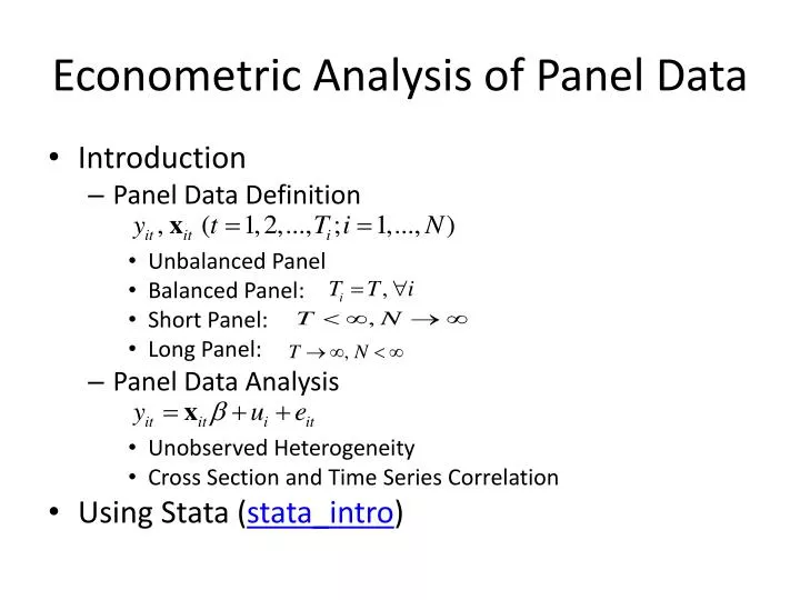
Econometric Analysis of Panel Data • Introduction • Panel Data Definition • Unbalanced Panel • Balanced Panel: • Short Panel: • Long Panel: • Panel Data Analysis • Unobserved Heterogeneity • Cross Section and Time Series Correlation • Using Stata (stata_intro)
Introduction • Panel Data • Definition (Wikipedia Encyclopedia) • Examples of Panel Datasets • Panel Study of Income Dynamics (PSID) • Penn World Table (PWT) • Panel Data Analysis • A Primer for Panel Data Analysis (Yaffee)
Using Stata • Declare Panel Data and Variables • xtset (or tsset) • xttab • Panel Data Analysis: xt commands • xtdes • xtsum • xtdata • xtline • Panel Data Regression • xtreg
Using Stata • Hypothesis Testing • xthausman • xttest0 • Advanced Topics • xtregar • xthtaylor (Hausman-Taylor Estimator) • xtivreg (Instrumental Variables Estimation) • xtabond (Arellano-Bond Estimator)
Example: Investment Demand • Grunfeld and Griliches [1960] • i = 10 firms: GM, CH, GE, WE, US, AF, DM, GY, UN, IBM; t = 20 years: 1935-1954 • Iit = Gross investment • Fit = Market value • Cit = Value of the stock of plant and equipment
Example: International Comparison of Economic Growth • R. Summers and A. Heston, "The Penn World Table (Mark 5): An Expanded Set of International Comparisons, 1950-1988," Quarterly Journal of Economics 106, 1991, 327-368. • G. Mankiw, D. Romer, and D. Weil, "A Contribution to the Empirics of Economic Growth,“ Quarterly Journal of Economics 107, 1992, 407-437.
Example: International Comparison of Economic Growth • yit = Real per capita GDP • si = Average saving rate (over 1960-1985) • ni = Average population growth rate (over 1960-1985) • g+d = 5% • COMi = 1 if communist, 0 otherwise • OPECi =1 if OPEC, 0 otherwise
Example: Returns to Schooling • Cornwell and Rupert Data, 595 Individuals, 7 Years • These data were analyzed in Cornwell, C. and Rupert, P., "Efficient Estimation with Panel Data: An Empirical Comparison of Instrumental Variable Estimators," Journal of Applied Econometrics, 3, 1988, pp. 149-155. See Baltagi, page 122 for further analysis.
Example: Returns to Schooling • LWAGE = log of wage = dependent variable in regressions • EXP = work experienceWKS = weeks workedOCC = occupation, 1 if blue collar, IND = 1 if manufacturing industrySOUTH = 1 if resides in southSMSA = 1 if resides in a city (SMSA)MS = 1 if marriedFEM = 1 if femaleUNION = 1 if wage set by union contractED = years of educationBLK = 1 if individual is black
Example: Wage Equation • Koop and Tobias [2004] • The data is available in two parts: • Part 1: Time-Variant Data (17,919 obs.) • id= Person id (ranging from 1 to 2178) • ed = Education • lwage = Log of hourly wage • pexp = Potential experience • trend = Time trend
Example: Wage Equation • Part 2: Time-Invariant Data (2178 individuals) • ability = Time invariant ability • medu = Mother’s education • fedu= Father’s education • d = Dummy variable for residence in a broken home • siblings = Number of siblings.
Example: U. S. Productivity • Munnell [1988] Productivity Data48 Continental U.S. States, 17 Years:1970-1986 • STATE = State name, • ST ABB=State abbreviation, • YR =Year, 1970, . . . ,1986, • PCAP =Public capital, • HWY =Highway capital, • WATER =Water utility capital, • UTIL =Utility capital, • PC =Private capital, • GSP =Gross state product, • EMP =Employment,