Download
1 / 35
350 likes | 472 Views
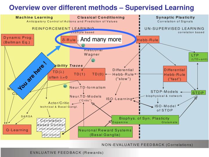
Overview over different methods – Supervised Learning. And many more. You are here !. u 1. Some more basics: Threshold Logic Unit (TLU). inputs. weights. w 1. output. activation. w 2. . u 2. v. q. a= i=1 n w i u i. w n. u n. 1 if a q v =

E N D
Overview over different methods – Supervised Learning And many more You are here !
u1 Some more basics:Threshold Logic Unit (TLU) inputs weights w1 output activation w2 u2 v . . . q a=i=1n wi ui wn un 1 if a q v= 0 if a< q {
Activation Functions threshold linear v v a a piece-wise linear sigmoid v v a a
Decision Surface of a TLU 1 1 Decision line w1 u1 + w2 u2 = q u2 > q 1 0 0 0 u1 1 0 0 < q
Scalar Products & Projections u u u w w w j j j w • v > 0 w • v = 0 w • v < 0 u w j w • u = |w||u| cos j
Geometric Interpretation The relation w•u=q implicitly defines the decision line u2 Decision line w1 u1 + w2 u2 = q w v=1 w•u=q |uw|=q/|w| uw u1 u v=0
Geometric Interpretation • In n dimensions the relation w•u=q defines a n-1 dimensional hyper-plane, which is perpendicular to the weight vector w. • On one side of the hyper-plane (w•u>q) all patterns are classified by the TLU as “1”, while those that get classified as “0” lie on the other side of the hyper-plane. • If patterns can be not separated by a hyper-plane then they cannot be correctly classified with a TLU.
Linear Separability u2 u2 w1=? w2=? q= ? w1=1 w2=1 q=1.5 0 1 0 1 u1 u1 1 0 0 0 Logical XOR Logical AND
u1 u2 un Threshold as Weight q=wn+1 1 if a 0 v= 0 if a<0 un+1=-1 w1 wn+1 w2 v . . . a= i=1n+1 wi ui wn {
Geometric Interpretation The relation w•u=0 defines the decision line u2 Decision line w w•u=0 v=1 u1 v=0 u
Training ANNs • Training set S of examples {u,vt} • u is an input vector and • vt the desired target output • Example: Logical And S = {(0,0),0}, {(0,1),0}, {(1,0),0}, {(1,1),1} • Iterative process • Present a training example u , compute network output v , compare output v with target vt, adjust weights and thresholds • Learning rule • Specifies how to change the weights w and thresholds q of the network as a function of the inputs u, output v and target vt.
Adjusting the Weight Vector u u w’ = w + mu j>90 mu w w Target vt =1 Output v=0 Move w in the direction of u u u w -mu j<90 w w’ = w - mu Target vt =0 Output v=1 Move w away from the direction of u
Perceptron Learning Rule • w’=w + m (vt-v) u Or in components • w’i = wi + Dwi = wi + m (vt-v) ui (i=1..n+1) With wn+1 = q and un+1=-1 • The parameter m is called the learning rate. It determines the magnitude of weight updates Dwi . • If the output is correct (vt=v) the weights are not changed (Dwi =0). • If the output is incorrect (vt v) the weights wi are changed such that the output of the TLU for the new weights w’i is closer/further to the input ui.
Perceptron Training Algorithm Repeat for each training vector pair (u, vt) evaluate the output y when u is the input if vvt then form a new weight vector w’ according to w’=w + m (vt-v) u else do nothing end if end for Until v=vt for all training vector pairs
Perceptron Convergence Theorem • The algorithm converges to the correct classification • if the training data is linearly separable • and m is sufficiently small • If two classes of vectors {u1} and {u2} are linearly separable, the application of the perceptron training algorithm will eventually result in a weight vector w0, such that w0 defines a TLU whose decision hyper-plane separates {u1} and {u2} (Rosenblatt 1962). • Solution w0 is not unique, since if w0 u =0 defines a hyper-plane, so does w’0= k w0.
Linear Separability u2 u2 w1=? w2=? q= ? w1=1 w2=1 q=1.5 0 1 0 1 u1 u1 1 0 0 0 Logical XOR Logical AND
Generalized Perceptron Learning Rule If we do not include the threshold as an input we use the follow description of the perceptron with symmetrical outputs (this does not matter much, though): Then we get for the learning rule: and This implies: Hence, if vt=1 and v=-1 the weight change increase the term w.u-q and vice versa. This is what we need to compensate the error!
u1 u2 un Linear Unit – no Threshold! inputs weights w1 output activation w2 v . . . v= a = i=1n wi vi a=i=1n wi ui wn Lets abbreviate the target output (vectors) by t in the next slides
Gradient Descent Learning Rule • Consider linear unit without threshold and continuous output v (not just –1,1) • v=w0 + w1 u1 + … + wn un • Train the wi’s such that they minimize the squared error • E[w1,…,wn] = ½ dD (td-vd)2 where D is the set of training examples and t the target outputs.
(w1,w2) Gradient: E[w]=[E/w0,… ,E/wn] (w1+w1,w2 +w2) Gradient Descent D={<(1,1),1>,<(-1,-1),1>, <(1,-1),-1>,<(-1,1),-1>} w=-m E[w] -1/m wi= - E/wi =/wi 1/2d(td-vd)2 = /wi 1/2d(td-i wi ui)2 = d(td- vd)(-ui)
Gradient Descent Gradient-Descent(training_examples, m) Each training example is a pair of the form {(u1,…un),t} where (u1,…,un) is the vector of input values, and t is the target output value, m is the learning rate (e.g. 0.1) • Initialize each wi to some small random value • Until the termination condition is met, Do • Initialize each wi to zero • For each {(u1,…un),t} in training_examples Do • Input the instance (u1,…,un) to the linear unit and compute the output v • For each linear unit weight wi Do • wi= wi + m (t-v) ui • For each linear unit weight wi Do • wi=wi+wi
This is the d-Rule Incremental Stochastic Gradient Descent • Batch mode : gradient descent w=w - m ED[w] over the entire data D ED[w]=1/2d(td-vd)2 • Incremental (stochastic) mode: gradient descent w=w - m Ed[w] over individual training examples d Ed[w]=1/2 (td-vd)2 Incremental Gradient Descent can approximate Batch Gradient Descent arbitrarily closely if m is small enough.
Perceptron vs. Gradient Descent Rule • perceptron rule w’i = wi + m (tp-vp) uip derived from manipulation of decision surface. • gradient descent rule w’i = wi + m (tp-vp) uip derived from minimization of error function E[w1,…,wn] = ½ p (tp-vp)2 by means of gradient descent.
Perceptron vs. Gradient Descent Rule Perceptron learning rule guaranteed to succeed if • Training examples are linearly separable • Sufficiently small learning rate m. Linear unit training rules using gradient descent • Guaranteed to converge to hypothesis with minimum squared error • Given sufficiently small learning rate m • Even when training data contains noise • Even when training data not separable by hyperplane.
Presentation of Training Examples • Presenting all training examples once to the ANN is called an epoch. • In incremental stochastic gradient descent training examples can be presented in • Fixed order (1,2,3…,M) • Randomly permutated order (5,2,7,…,3) • Completely random (4,1,7,1,5,4,……)
x1 x2 xn Neuron with Sigmoid-Function inputs weights w1 output activation w2 y . . . a=i=1n wi xi wn y=s(a) =1/(1+e-a)
u1 u2 un Sigmoid Unit x0=-1 w1 w0 a=i=0n wi ui v=(a)=1/(1+e-a) w2 v . . . (x) is the sigmoid function: 1/(1+e-x) wn d(x)/dx= (x) (1- (x)) • Derive gradient decent rules to train: • one sigmoid function • E/wi = -p(tp-v) v(1-v) uip • Multilayer networks of sigmoid units • backpropagation:
Gradient Descent Rule for Sigmoid Output Function s sigmoid Ep[w1,…,wn] = ½ (tp-vp)2 Ep/wi = /wi ½ (tp-vp)2 = /wi ½ (tp- s(Si wi uip))2 = (tp-up) s‘(Si wi uip) (-uip) for v=s(a) = 1/(1+e-a) s’(a)= e-a/(1+e-a)2=s(a) (1-s(a)) a s’ a w’i= wi + wi = wi + m v(1-v)(tp-vp) uip
Gradient Descent Learning Rule vj wi = m vjp(1-vjp) (tjp-vjp) uip wji ui activation of pre-synaptic neuron learning rate error djof post-synaptic neuron derivative of activation function
ALVINN Automated driving at 70 mph on a public highway Camera image 30 outputs for steering 30x32 weights into one out of four hidden unit 4 hidden units 30x32 pixels as inputs