Download
1 / 50
520 likes | 769 Views
Sparse Matrix Methods on High Performance Computers. X. Sherry Li xsli@lbl.gov http://crd.lbl.gov/~xiaoye CS267/EngC233: Applications of Parallel Computers March 16, 2010. Sparse linear solvers . . . for unstructured matrices. Solving a system of linear equations Ax = b Iterative methods

E N D
Sparse Matrix Methods on High Performance Computers X. Sherry Li xsli@lbl.gov http://crd.lbl.gov/~xiaoye CS267/EngC233: Applications of Parallel Computers March 16, 2010
Sparse linear solvers . . . for unstructured matrices • Solving a system of linear equations Ax = b • Iterative methods • A is not changed (read-only) • Key kernel: sparse matrix-vector multiply • Easier to optimize and parallelize • Low algorithmic complexity, but may not converge for hard problems • Direct methods • A is modified (factorized) • Harder to optimize and parallelize • Numerically robust, but higher algorithmic complexity • Often use direct method to precondition iterative method • Increasingly more interest on hybrid methods
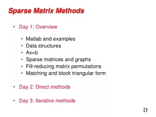
Lecture Plan • Direct methods . . . Sparse factorization • Sparse compressed formats • Deal with many graph algorithms: directed/undirected graphs, paths, elimination trees, depth-first search, heuristics for NP-hard problems, cliques, graph partitioning, cache-friendly dense matrix kernels, and more . . . • Preconditioners . . . Incomplete factorization • Hybrid method . . . Domain decomposition
Available sparse factorization codes • Survey of different types of factorization codes http://crd.lbl.gov/~xiaoye/SuperLU/SparseDirectSurvey.pdf • LLT (s.p.d.) • LDLT (symmetric indefinite) • LU (nonsymmetric) • QR (least squares) • Sequential, shared-memory (multicore), distributed-memory, out-of-core • Distributed-memory codes: usually MPI-based • SuperLU_DIST [Li/Demmel/Grigori] • accessible from PETSc, Trilinos • MUMPS, PasTiX, WSMP, . . .
Review of Gaussian Elimination (GE) • First step of GE: • Repeats GE on C • Results in LU factorization (A = LU) • L lower triangular with unit diagonal, U upper triangular • Then, x is obtained by solving two triangular systems with L and U
U 1 2 3 4 L 5 6 7 Sparse GE • Sparse matrices are ubiquitous • Example: A of dimension 106, 10~100 nonzeros per row • Nonzero costs flops and memory • Scalar algorithm: 3 nested loops • Can re-arrange loops to get different variants: left-looking, right-looking, . . . for i = 1 to n column_scale ( A(:,i) ) for k = i+1 to n s.t. A(i,k) != 0 for j = i+1 to n s.t. A(j,i) != 0 A(j,k) = A(j,k) - A(j,i) * A(i,k) Typical fill-ratio: 10x for 2D problems, 30-50x for 3D problems
Early Days . . . Envelope (Profile) solver • Define bandwidth for each row or column • A little more sophisticated than band solver • Use Skyline storage (SKS) • Lower triangle stored row by row Upper triangle stored column by column • In each row (column), first nonzero defines a profile • All entries within the profile (some may be zeros) are stored • All fill-ins are confined in the profile • A good ordering would be based on bandwidth reduction • E.g., (reverse) Cuthill-McKee
RCM ordering • Breadth-first search, numbering by levels, then reverse
Example: 3 orderings (natural, RCM, Minimum-degree) Envelop size = sum of bandwidths After LU, envelop would be entirely filled Is Profile Solver Good Enough? Env = 61066 NNZ(L, MD) = 12259 Env = 31775 Env = 22320 9
nzval 1 c 2 d e 3 k a 4 h b f 5 i l 6 g j 7 rowind 1 3 2 3 4 3 7 1 4 6 2 4 5 6 7 6 5 6 7 colptr 1 3 6 8 11 16 17 20 A General Data Structure: Compressed Column Storage (CCS) • Also known as Harwell-Boeing format • Store nonzeros columnwise contiguously • 3 arrays: • Storage: NNZ reals, NNZ+N+1 integers • Efficient for columnwise algorithms • “Templates for the Solution of Linear Systems: Building Blocks for Iterative Methods”, R. Barrett et al.
General Sparse Solver • Use (blocked) CRS or CCS, and any ordering method • Leave room for fill-ins ! (symbolic factorization) • Exploit “supernodal” (dense) structures in the factors • Can use Level 3 BLAS • Reduce inefficient indirect addressing (scatter/gather) • Reduce graph traversal time using a coarser graph 11
Numerical Stability: Need for Pivoting • One step of GE: • If α is small, some entries in B may be lost from addition • Pivoting: swap the current diagonal entry with a larger entry from the other part of the matrix • Goal: prevent from getting too large
x s x x b x x x Dense versus Sparse GE • Dense GE: Pr A Pc = LU • Pr and Pc are permutations chosen to maintain stability • Partial pivoting suffices in most cases : Pr A = LU • Sparse GE: Pr A Pc = LU • Pr and Pc are chosen to maintain stability and preserve sparsity, and increase parallelism • Dynamic pivoting causes dynamic structural change • Alternatives: threshold pivoting, static pivoting, . . .
Algorithmic Issues in Sparse GE • Minimize number of fill-ins, maximize parallelism • Sparsity structure of L & U depends on that of A, which can be changed by row/column permutations (vertex re-labeling of the underlying graph) • Ordering (combinatorial algorithms; NP-complete to find optimum [Yannakis ’83]; use heuristics) • Predict the fill-in positions in L & U • Symbolic factorization (combinatorial algorithms) • Perform factorization and triangular solutions • Numerical algorithms (F.P. operations only on nonzeros) • How and when to pivot ? • Usually dominate the total runtime
Ordering • RCM is good for profile solver • General unstructured methods: • Minimum degree (locally greedy) • Nested dissection (divided-conquer, suitable for parallelism)
i j k l 1 i j k 1 l i i j j k k l l Ordering : Minimum Degree (1/3) Local greedy: minimize upper bound on fill-in i j k l 1 i Eliminate 1 j k l Eliminate 1
Minimum Degree Ordering (2/3) • At each step • Eliminate the vertex with the smallest degree • Update degrees of the neighbors • Greedy principle: do the best locally • Best for modest size problems • Hard to parallelize • Straightforward implementation is slow and requires too much memory • Newly added edges are more than eliminated vertices
Minimum Degree Ordering (3/3) • Use quotient graph as a compact representation [George/Liu ’78] • Collection of cliques resulting from the eliminated vertices affects the degree of an uneliminated vertex • Represent each connected component in the eliminated subgraph by a single “supervertex” • Storage required to implement QG model is bounded by size of A • Large body of literature on implementation variants • Tinney/Walker `67, George/Liu `79, Liu `85, Amestoy/Davis/Duff `94, Ashcraft `95, Duff/Reid `95, et al., . .
Nested Dissection Ordering (1/3) • Model problem: discretized system Ax = b from certain PDEs, e.g., 5-point stencil on k x k grid, N = k^2 • Theorem: NDordering gave optimal complexity in exact arithmetic [George ’73, Hoffman/Martin/Rose, Eisenstat, Schultz and Sherman] • 2D (kxk = N grids): O(N logN) memory, O(N3/2) operations • 3D (kxkxk = N grids): O(N4/3) memory, O(N2) operations
ND Ordering (2/3) • Generalized nested dissection [Lipton/Rose/Tarjan ’79] • Global graph partitioning: top-down, divide-and-conqure • Best for largest problems • Parallel codes available: e.g., ParMetis, Scotch • First level • Recurse on A and B • Goal: find the smallest possible separator S at each level • Multilevel schemes: • Chaco [Hendrickson/Leland `94], Metis [Karypis/Kumar `95] • Spectral bisection [Simon et al. `90-`95] • Geometric and spectral bisection [Chan/Gilbert/Teng `94] A S B
Ordering for LU (unsymmetric) • Can use a symmetric ordering on a symmetrized matrix • Case of partial pivoting (sequential SuperLU): Use ordering based on ATA • Case of static pivoting (SuperLU_DIST): Use ordering based on AT+A • Can find better ordering based solely on A • Diagonal Markowitz [Amestoy/Li/Ng ‘06] • Similar to minimum degree, but without symmetrization • Hypergraph partition [Boman, Grigori, et al., ‘09] • Similar to ND on ATA,but no need to compute ATA
High Performance Issues: Reduce Cost of Memory Access & Communication • Blocking to increase flops-to-bytes ratio • Aggregate small messages into one larger message • Reduce cost due to latency • Well done in LAPACK, ScaLAPACK • Dense and banded matrices • Adopted in the new generation sparse software • Performance much more sensitive to latency in sparse case
Source of parallelism (1): Elimination Tree • For any ordering . . . • A column a vertex in the tree • Exhibits column dependencies during elimination • If column j updates column k, then vertex j is a descendant of vertex k • Disjoint subtrees can be eliminated in parallel • Almost linear algorithm to compute the tree
Source of parallelism (2): Separator Tree • Ordering by graph partitioning
Source of parallelism (3): global partition and distribution • 2D block cyclic recommended for many linear algebra algorithms • Better load balance, less communication, and BLAS-3 1D blocked 1D cyclic 1D block cyclic 2D block cyclic
Major stages of sparse LU • Ordering • Symbolic factorization • Numerical factorization – usually dominates total time • How to pivot? • Triangular solutions • SuperLU_MT • 1. Sparsity ordering • 2.Factorization (steps interleave) • Partial pivoting • Symb. fact. • Num. fact. (BLAS 2.5) • 3. Solve SuperLU_DIST 1.Static pivoting 2. Sparsity ordering 3. Symbolic fact. 4. Numerical fact. (BLAS 3) 5. Solve
P1 P2 U A L NOT TOUCHED DONE BUSY SuperLU_MT [Li/Demmel/Gilbert] • Pthreads or OpenMP • Left looking -- many more reads than writes • Use shared task queue to schedule ready columns in the elimination tree (bottom up)
Matrix 2 2 Process mesh 4 5 4 5 0 2 2 2 4 5 4 5 4 5 2 2 4 5 4 5 2 SuperLU_DIST[Li/Demmel/Grigori] • MPI • Right looking -- many more writes than reads • Global 2D block cyclic layout, compressed blocks • One step look-ahead to overlap comm. & comp. 0 1 0 1 0 1 3 3 3 3 0 1 0 1 0 3 3 3 0 1 0 1 0 3 3 3 0 1 2 0 1 0 ACTIVE
Multicore platforms • Intel Clovertown: • 2.33 GHz Xeon, 9.3 Gflops/core • 2 sockets X 4 cores/socket • L2 cache: 4 MB/2 cores • Sun VictoriaFalls: • 1.4 GHz UltraSparc T2, 1.4 Gflops/core • 2 sockets X 8 cores/socket X 8 hardware threads/core • L2 cache shared: 4 MB
Clovertown • Maximum speedup 4.3, smaller than conventional SMP • Pthreads scale better • Question: tools to analyze resource contention
VictoriaFalls – multicore + multithread SuperLU_MT SuperLU_DIST • Maximum speedup 20 • Pthreads more robust, scale better • MPICH crashes with large #tasks, • mismatch between coarse and fine grain models 33
Larger matrices • Sparsity ordering: MeTis applied to structure of A’+A
Strong scaling: Cray XT4 (2.3 GHz) • Up to 794 Gflops factorization rate
Weak scaling • 3D KxKxK cubic grids, scale N2 = K6 with P for constant-work-per-processor • Performance sensitive to communication latency • Cray T3E latency: 3 microseconds ( ~ 2700 flops, 450 MHz, 900 Mflops) • IBM SP latency: 8 microseconds ( ~ 11940 flops, 1.9 GHz, 7.6 Gflops)
Analysis of scalability and isoefficiency • Model problem: matrix from 11 pt Laplacian on k x k x k (3D) mesh; Nested dissection ordering • N = k3 • Factor nonzeros (Memory) : O(N4/3) • Number of flops (Work) : O(N2) • Total communication overhead : O(N4/3 P) (assuming P processors arranged as grid) • Isoefficiency function: Maintain constant efficiency if “Work” increases proportionally with “Overhead”: This is equivalent to: • Memory-processor relation: • Parallel efficiency can be kept constant if the memory-per-processor is constant, same as dense LU in ScaLPAPACK • Work-processor relation: • Work needs to grow faster than processors
Incomplete factorization (ILU) preconditioner • A very simplified view: • Structure-based dropping: level of fill • ILU(0), ILU(k) • Rationale: the higher the level, the smaller the entries • Separate symbolic factorization step to determine fill-in pattern • Value-based fropping: drop truly small entries • Fill-in pattern must be determined on-the-fly • ILUTP [Saad]: among the most sophisticated, and (arguably) robust • “T” = threshold, “P” = pivoting • Implementation similar to direct solver • We use SuperLU code base to perform ILUTP
SuperLU [Demmel/Eisenstat/Gilbert/Liu/Li ’99]http://crd.lbl.gov/~xiaoye/SuperLU • Left-looking, supernode • Sparsity ordering of columns • use graph of A’*A • Factorization • For each panel … • Partial pivoting • Symbolic fact. • Num. fact. (BLAS 2.5) • Triangular solve panel U A L NOT TOUCHED DONE WORKING
Primary dropping rule: S-ILU(tau) [Li/Shao ‘09] • Similar to ILUTP, adapted to supernode • U-part: • L-part: retain supernode • Compare with scalar ILU(tau) • For 54 matrices, S-ILU+GMRES converged with 47 cases, versus 43 with scalar ILU+GMRES • S-ILU +GMRES is 2.3x faster than scalar ILU+GMRES i
Secondary dropping rule: S-ILU(tau,p) • Control fill ratio with a user-desired upper bound • Earlier work, column-based • [Saad]: ILU(tau, p), at most p largest nonzeros allowed in each row • [Gupta/George]: p adaptive for each column May use interpolation to compute a threshold function, no sorting • Our new scheme is “area-based” • Define adaptive upper bound function • More flexible, allow some columns to fill more, but limit overall j+1
Experiments: GMRES + ILU • Use restarted GMRES with our ILU as a right preconditioner • Size of Krylov subspace set to 50 • Stopping criteria:
S-ILU for extended MHD (plasma fusion engery) • Opteron 2.2 GHz (jacquard at NERSC), one processor • ILU parameters: drop_tol = 1e-4, gamma = 10 • Up to 9x smaller fill ratio, and 10x faster
Compare with other ILU codes • SPARSKIT 2 : scalar version of ILUTP [Saad] • ILUPACK 2.3 : inverse-based multilevel method [Bolhoefer et al.] • 232 test matrices : dimension 5K-1M • Performance profile of runtime – fraction of the problems a solver could solve within a multiple of X of the best solution time among all the solvers • S-ILU succeeded with 141 ILUPACK succeeded with 130 Both succeeded with 99
Hybrid solver – Schur complement method • Schur complement method • a.k.a. iterative substructuring method • a.k.a. non-overlapping domain decomposition • Partition into many subdomains • Direct method for each subdomain, perform partial elimination independently, in parallel • Preconditioned iterative method for the Schur complement system, which is often better conditioned, smaller but denser
Structural analysis view • Case with two subdomains Substructure contribution: Interface
Parallelism – multilevel partitioning • Nested dissection, graph partitioning • Memory requirement: fill is restricted within • “small” diagonal blocks of A11, and • ILU(S), sparsity can be enforced • Two levels of parallelism: can use lots of processors • multiple processors for each subdomain direct solution • only need modest level of parallelism from direct solver • multiple processors for interface iterative solution
Parallel performance on Cray XT4 [Yamazaki/Li ‘10] • Omega3P to design ILC accelerator cavity (Rich Lee, SLAC) • Dimension: 17.8 M, real symmetric, highly indefinite • PT-SCOTCH to extract 64 subdomains of size ~ 277K. The Schur complement size is ~ 57K • SuperLU_DIST to factorize each subdomain • BiCGStab of PETSc to solve the Schur system, with LU(S1) preconditioner • Converged in ~ 10 iterations, with relative residual < 1e-12
Summary • Sparse LU, ILU are important kernels for science and engineering applications, used in practice on a regular basis • Good implementation on high-performance machines requires a large set of tools from CS and NLA • Performance more sensitive to latency than dense case
Open problems • Much room for optimizing performance • Automatic tuning of blocking parameters • Use of modern programming language to hide latency (e.g., UPC) • Scalability of sparse triangular solve • Switch-to-dense, partitioned inverse • Parallel ILU • Optimal complexity sparse factorization • In the spirit of fast multipole method, but for matrix inversion • J. Xia’s dissertation (May 2006) • Latency-avoiding sparse factorizations