Download
1 / 29
320 likes | 427 Views
Introduction to Financial Economics. Lecture Notes 5 Ch.5-Lengwiler. Overview of the Course. Introduction- Finance and Economic theory- general equilibrium and macroeconomic foundations. Contingent Claim Economies - Commodity spaces, preferences, general equilibrium, representative agents.

E N D
Introduction to Financial Economics Lecture Notes 5 Ch.5-Lengwiler
Overview of the Course • Introduction- Finance and Economic theory- general equilibrium and macroeconomic foundations. • Contingent Claim Economies - Commodity spaces, preferences, general equilibrium, representative agents. • Asset Economies- financial assets, Radner economies, Arrow-Debreu pricing, complete and incomplete markets. • Risky Decisions- expected utility paradigm. • Static Finance Economy- risk sharing, representative vNM agent, sdf’s, equilibrium price of risk and time. • Dynamic Finance Economies- dynamic trading etc. • Taking Theory to the Data: Empirical Applications.
Arrow-Debreu general equilibrium, welfare theorem, representative agent Radner economies real/nominal assets, market span, representative good von Neumann Morgenstern measures of risk aversion, HARA class von Neumann Morgenstern measures of risk aversion, HARA class Finance economy Risk Sharing SDF’s etc The Big Picture Data and the Puzzles Empirical resolutions Theoretical resolutions
A Finance Economy • Combines Arrow-Debreu-Radner economy with vNM expected utility theory. • Finance economy- built on GE theory + vNM utility theory. • Why do this? • To obtain empirically testable asset pricing formulae. • To study how much is society is willing to pay for a marginal reduction of risk- or the welfare implications of risks in the economy. • How to do this? • To apply vNM theory to a GE model we need • To treat assets as lotteries • make assumptions that allows consideration of the utility of consumption now and tomorrow (two-period world).
Combining vNM EU theory and GE-I • In vNM world- a risky decision is characterized by the agent’s vNM utility function v, her initial wealth (w) and the lottery [x11,…, xSS]under review. • Objective function is : • If wealth is viewed as state contingent, the objective is the expected utility of state-contingent wealth or (w+x1,w+x2…w+xS). • Adapting this with a GE model requires two things: • Capture uncertainty in the economy not by an arbitrary set of lotteries or gambles but • Instead used the idea of states of the world to model uncertainty.
Combining vNM EU theory and GE-II • We restrict the set of vNM lotteries to include only lotteries with S possible outcomes and a fixed probability distribution over these outcomes. • Distribution over outcomes corresponds to the probability distribution of the states of the world. • Asset a lottery that assigns different payoffs, xs to different states of the world. • Portfolio of assets mixture of lotteries. • Our GE model specifies two periods: • Agents can choose how much to allocate to different states tomorrow (across states) but also how much to consume now and tomorrow (over time).
EU over two periods-I • We do this by using a vNM utility function that is additively separable over time. • There is a vNM utility function: • v, that maps today’s consumption to today’s utility. • u, maps tomorrow’s consumption to tomorrow’s utility. • Total expected utility is : • Need to model how our utility function changes through time. • We assume that utility is additively separable through time. • We assume that v and u are equal in terms of risk aversion- u is a linear transformation of v.
EU over two periods-II • We let: u(y)= v(y). • Here is the time preference parameter-we also assume 1 or consumption today is valued more than consumption tomorrow. • Agent maximizes: • So now we have: • An agent i, with vNM utility vi, impatience i and state-contingent income tomorrow w(i). • If we let different agents in the economy have different beliefs i. • We also assume asset markets are complete i.e. the return matrix is invertible or it could be be replaced by an identity matrix- there is a market for each Arrow security. • Economy described by: vi,i, i. wi; r the return matrix or now e: the AD matrix.
Portfolio problem- with vNM agents I • Income tomorrow is uncertain or state-contingent (a lottery). • Problem for the individual: • How much to save today? • How to insure your income tomorrow? • Wish to move wealth through time (save or borrow). • Wish to move across states (insure or take bets). • Decision problem of a vNM agent in a finance economy is :
The Portfolio problem-II • We can write this more compactly as: • For Equilibrium: • W and Y; the aggregate endowment and consumption. • The Radner equilibrium of this asset economy is a pair consisting of a price for each asset , and an allocation (y(1), ..,y(I)), such that y(i) solves the above optimization problem for each i and all market clear or Y-W=0.
How do we deal with agent’s beliefs? • We have allowed for agents in our model to have different beliefs about the states of the world tomorrow. • Suppose there is a true objective probability distribution over the states of the world –but this is not known. • Each agent receives an imperfect signal about the true distribution. • Agent’s signal is correlated with true distribution plus some noise. • Its thus important to know not only your distribution but also that of others in order to improve your ability to judge the true distribution. • Valuable to have your opinion- but also important to know other people’s opinion.
Common Beliefs-I • Suppose every agent uses her own assessment of probabilities to maximize her expected utility- resulting equilibrium prices will contain information about the average opinion of the other agents. • Implies that every agent will want to revise their probability assessments. • We have allowed for agents in our model to have different beliefs about the states of the world tomorrow. • Our definition of equilibrium is incomplete- we need a combination of allocation, prices and beliefs-so that all markets clear and there is no incentive to revise beliefs. • How do we tackle this? – by simply assuming that everyone has the same beliefs.
Common Beliefs-II • In this equilibrium prices will be compatible with common beliefs-no one will need to revise them. • Fully revealing REE- Radner equilibrium of an economy with heterogeneous beliefs- which is such that market prices are a sufficient statistic for all information of all agents. • This is a strong assumption but not making it make for complicated models because prices have two roles: • Measuring scarcity of goods. • Conveying private information to the public. • We assume that “market prices” are a sufficient statistic for the information of all agents • Agents simply use this common information and ignore private information completely. • This is called a Fully Revealing REE in the literature.
Common Beliefs- III • In this equilibrium it seems rational for an agent to use the commonly available information in decision-making and to completely ignore his private information. • Suppose all agents ignored private information- then how can prices be affected i.e. by information that everyone has- this is the Grossman-Stiglitz paradox- we will not pursue this here. • We now assume common beliefs, and define beliefs as a part of the economy not as a property of an agent. • Now on we have an agent with intertemporal vNM utility is a triple (vi,I,w(i)) and an economy is the collection of all agents, plus beliefs and an asset matrix:
Common Beliefs- IV • In this equilibrium it seems rational for an agent to use the commonly available information in decision-making and to completely ignore his private information. • Suppose all agents ignored private information- then how can prices be affected i.e. by information that everyone has- this is the Grossman-Stiglitz paradox- we will not pursue this here. • We now assume common beliefs, and define beliefs as a part of the economy not as a property of an agent. • Now on we have an agent with intertemporal vNM utility is a triple (vi,I,w(i)) and an economy is the collection of all agents, plus beliefs and an asset matrix:
Risk Sharing-I • We now focus on the main theme of all the research papers that form a part of the reading and the assessment for this course. • The main point is the following: • If preferences are time separable and display weak aversion. • If all individuals discount the future at the same rate. • All information is held in common. • Then an optimal allocation of risk bearing of a single good in a uncertain environment is one where all individual consumptions are determined by aggregate consumption- no matter what the date and history of shocks- so individual consumptions will move together. • An important paper is Wilson (1968) which makes two points: • Mutuality Principle: An efficient allocation of resources requires that only aggregate risk be borne by the agents- all idiosyncratic risk can be diversified away by mutual insurance among agents. • Allocation of aggregate risk between agents: Marginal aggregate risk borne by an agent equals the ration of her absolute risk tolerance to the average risk tolerance of the population.
Risk Sharing • Suppose two states have the same aggregate endowment-though they may differ with respect to the state-contingent distribution of income among agents. • Such states differ only with respect to idiosyncratic risk- no aggregate risk between them- an efficient allocation implies that everyone should consume the same in both states. Mutuality Principle (Wilson, 1968) An efficient allocation of resources requires that only aggregate risk be borne by the agents- all idiosyncratic risk can be diversified away by mutual insurance among agents. • Agents should only bet on aggregate risk- an individuals consumption is a function of aggregate endowment only. • We will not go into the proof here-take it as given-consequence of 2nd Welfare Theorem.
Empirical Evidence on Risk Sharing • Many empirical papers have looked at the ways in which risk is shared from village economies, to regions and between countries. • Some examples are: • Townsend- Village Economies • Asdrubali, Sorensen and Yosha- Regions and Countries • Cochrane and Mace – Empirics of Consumption Risk Sharing • Van Wincoop – International Risk Sharing • In the homework for this course you will be required to read one of these papers and provide a critical review of its contribution. • We now look at Wilson’s second result-how aggregate risk is shared between agents.
Allocation of aggregate risk among agents • We know from the mutuality principle that in an efficient allocation people bear only aggregate risk. • But who bears this risk- How is the burden of aggregate risk allocated among the agents? • We can get an insight by looking at the weights in the Social Welfare function. • We know from the SWF that for every Pareto efficient allocation there is a vector of weights, one for each agent- with vNM agents and common beliefs the SWF is :
The Social Welfare function • This objective function is additively separable between states and there is one constraint for each state. • We can thus write this problem as a sum of simple one-dimensional maximization problems
Second Result of Wilson (1968) • Consider • The FOC is : • Here is the LM of the feasibility constraint- measures the marginal increase in u when the constraint is marginally eased-expanding z by dz and eases the constraint I times dz:
Wilson’s Theorem-II • Solving for i’s marginal share of the aggregate risk yields: • But • Thus • Where Ti is i’s absolute tolerance and T is the tolerance associated with the utility function u- the marginal share of the aggregate risk borne by an agent I is proportional to the agent’s absolute risk tolerance.
Wilson’s Theorem-II • We require that the average change of consumption dy(i) equals the change of per capita endowment dz. • Taking averages of the following we get: • The risk tolerance u is the average risk tolerance of the population. • Wilson (1968) result: The marginal aggregate risk borne by an agent equals the ratio of his absolute risk tolerance to the average risk tolerance of the population.
Distribution Independent Aggregation • The R.A’s tastes depend on all aspects of the economy including inter-personal income distribution. • Thus asset prices will depend nor only on aggregate endowment but on the distribution as well. • What assumptions are required to make the representative agent’s utility independent of the distribution? • Rubinstein (1974) shows that if individuals have HARA utility with a quantity defined as common cautiousness then the R.A’s utility does not depend on the distribution of income. • This results from an application of Wilson’s theorem.
Quasi-Complete Markets • Under some special conditions- we can have equilibrium allocations that are Pareto efficient even if the market is incomplete and hence aggregation can be performed. • By Mutuality- only aggregate risk is important. • If the market allows each individual to hedge his idiosyncratic risk by buying some aggregate endowment in each state and • Also allows each agent to allocate their consumption through time according to their time preferences, then the market is quasi-complete. • Sufficient conditions for quasi-completeness (Ross, 1976) • If agents i’s future contingent income wi is in the asset span, so that each agent can sell or buy a fraction of his idiosyncratic risk • if there is a complete set of call options on the aggregate endowment.
The SDF and the MRS • The representative agent’s portfolio problem is : • We know that the equilibrium net trade of the representative is zero. Thus the FOC must be satisfied at the endowment point: • Thus if (v,,w) is a vNM representative then, in equilibrium: • Thus the SDF is the MRS x rate of time presence- stochastic because it is so + discount because it is like a PV factor.
Manipulating the SDF-Equilibrium Price of Risk • Now we show that simple manipulation of the fundamental asset pricing equation gives us a range of insights. • Start with the covariance decomposition: • CCAPM: In equilibrium the SDF is given by the FOC of the portfolio problem of the representative:
Equilibrium Price of Risk-I • If the rate of return of an asset is not correlated with aggregate risk, then the risk premium is zero and the expected return on this asset equals the risk-free rate. Why? • Any risk inherent in this asset can be diversified away since it is not related to aggregate risk. • The risk of this asset will not be borne by anyone, in an efficient allocation, (by the Mutuality Principle) and thus has no effect on the price of the asset. • An asset whose return covaries positively with aggregate endowment will carry a positive risk premium. Why? • This asset pays out in good times and fails to payoff in bad times- thus we need an incentive or a positive risk premium to hold such an asset.
Equilibrium Price of Risk-II • An asset whose return covaries negatively with aggregate endowment is a hedge against aggregate risk-it can be used to ensure against aggregate risk. • Of course such insurance is nor possible for the aggregate but this asset allows the owner to pass on the aggregate risk to other agents. • Hence such assets are valuable and carry a negative risk premium. • Many aspects that we have not covered: • Proof of Wilson’s theorems. • Proof of Rubinstein (1974) about the conditions under which equilibrium prices are independent from inter-personal income distribution. • However now it is time to look at some applications.