Download
1 / 19
190 likes | 344 Views
QUIZ!!. T/F: The forward algorithm is really variable elimination, over time. TRUE T/F: Particle Filtering is really sampling, over time. TRUE T/F: In HMMs, each variable X i has its own (different) CPT. FALSE T/F: In the forward algorithm, you must normalize each iteration. FALSE

E N D
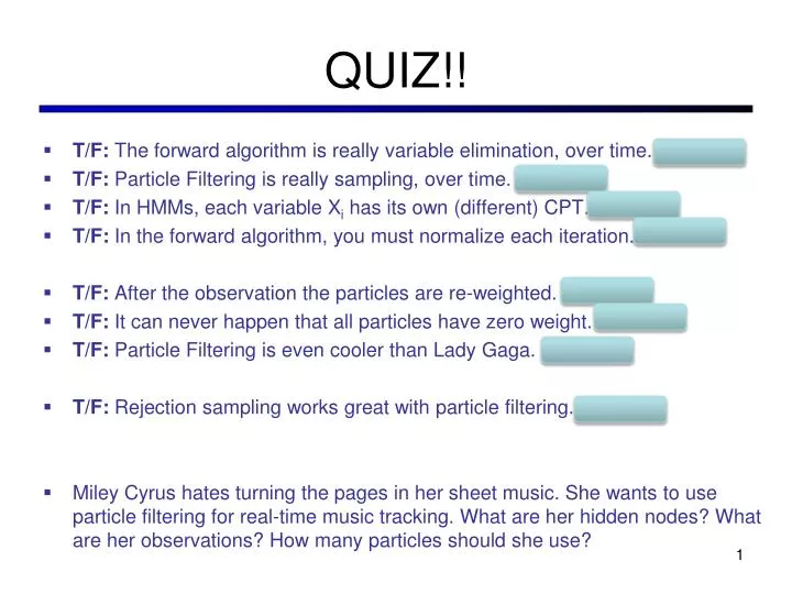
QUIZ!! • T/F: The forward algorithm is really variable elimination, over time. TRUE • T/F: Particle Filtering is really sampling, over time. TRUE • T/F: In HMMs, each variable Xi has its own (different) CPT. FALSE • T/F: In the forward algorithm, you must normalize each iteration. FALSE • T/F: After the observation the particles are re-weighted. TRUE • T/F: It can never happen that all particles have zero weight. FALSE • T/F: Particle Filtering is even cooler than Lady Gaga. TRUE • T/F: Rejection sampling works great with particle filtering. FALSE • Miley Cyrus hates turning the pages in her sheet music. She wants to use particle filtering for real-time music tracking. What are her hidden nodes? What are her observations? How many particles should she use?
CSE 511a: Artificial IntelligenceSpring 2013 Lecture 21: Particles++ April 17, 2013 Robert Pless, Via KilianQ. Weinberger, with slides adapted from Dan Klein – UC Berkeley
Announcements • Project 4 due Monday April 22 • HW2 out today! due 10am Monday April 29 • Posted online. • Any group size. • Same deal as HW before midterm • Contest out soon! • Groups of <= 5. • Extra Credit points awarded for achievements (beat baseline algorithm, ever being first, being first at particular checkpoints). • Contest ends Sunday May 4, 5pm. • Grade checkpoint available soon (sorry).
0.0 0.1 0.0 0.0 0.0 0.2 0.0 0.2 0.5 Particle Filtering • Sometimes |X| is too big to use exact inference • |X| may be too big to even store B(X) • E.g. X is continuous • |X|2 may be too big to do updates • Solution: approximate inference • Track samples of X, not all values • Samples are called particles • Time per step is linear in the number of samples • But: number needed may be large • In memory: list of particles, not states • This is how robot localization works in practice
Representation: Particles • Our representation of P(X) is now a list of N particles (samples) • Generally, N << |X| • Storing map from X to counts would defeat the point • P(x) approximated by number of particles with value x • So, many x will have P(x) = 0! • More particles, more accuracy • For now, all particles have a weight of 1 Particles: (3,3) (2,3) (3,3) (3,2) (3,3) (3,2) (2,1) (3,3) (3,3) (2,1)
Particle Filtering: Elapse Time • Each particle is moved by sampling its next position from the transition model • This is like prior sampling – samples’ frequencies reflect the transition probs • Here, most samples move clockwise, but some move in another direction or stay in place • This captures the passage of time • If we have enough samples, close to the exact values before and after (consistent)
Particle Filtering: Observe • Slightly trickier: • We don’t sample the observation, we fix it • This is similar to likelihood weighting, so we downweight our samples based on the evidence • Note that, as before, the probabilities don’t sum to one, since most have been downweighted (in fact they sum to an approximation of P(e))
Particle Filtering: Resample Old Particles: (3,3) w=0.1 (2,1) w=0.9 (2,1) w=0.9 (3,1) w=0.4 (3,2) w=0.3 (2,2) w=0.4 (1,1) w=0.4 (3,1) w=0.4 (2,1) w=0.9 (3,2) w=0.3 • Rather than tracking weighted samples, we resample • N times, we choose from our weighted sample distribution (i.e. draw with replacement) • This is equivalent to renormalizing the distribution • Now the update is complete for this time step, continue with the next one Old Particles: (2,1) w=1 (2,1) w=1 (2,1) w=1 (3,2) w=1 (2,2) w=1 (2,1) w=1 (1,1) w=1 (3,1) w=1 (2,1) w=1 (1,1) w=1
Particle Filters for Localization and Video Tracking • http://www.youtube.com/watch?v=wCMk-pHzScE
Dynamic Bayes Nets (DBNs) • We want to track multiple variables over time, using multiple sources of evidence • Idea: Repeat a fixed Bayes net structure at each time • Variables from time t can condition on those from t-1 • Discrete valued dynamic Bayes nets are also HMMs t =1 t =2 t =3 G1a G2a G3a G1b G2b G3b E1a E1b E2a E2b E3a E3b
Exact Inference in DBNs • Variable elimination applies to dynamic Bayes nets • Procedure: “unroll” the network for T time steps, then eliminate variables until P(XT|e1:T) is computed • Online belief updates: Eliminate all variables from the previous time step; store factors for current time only t =3 t =1 t =2 G3a G1a G2a G3b G3b G1b G2b E3a E3b E1a E1b E2a E2b
DBN Particle Filters • A particle is a complete sample for a time step • Initialize: Generate prior samples for the t=1 Bayes net • Example particle: G1a = (3,3) G1b = (5,3) • Elapse time: Sample a successor for each particle • Example successor: G2a = (2,3) G2b = (6,3) • Observe: Weight each entire sample by the likelihood of the evidence conditioned on the sample • Likelihood: P(E1a |G1a ) * P(E1b |G1b ) • Resample: Select prior samples (tuples of values) in proportion to their likelihood
Best Explanation Queries [video] • Query: most likely seq: X1 X2 X3 X4 X5 E1 E2 E3 E4 E5
HMMs: MLE Queries • HMMs defined by • States X • Observations E • Initial distr: • Transitions: • Emissions: • Query: most likely explanation: X1 X2 X3 X4 X5 E1 E2 E3 E4 E5
State Path Trellis • State trellis: graph of states and transitions over time • Each arc represents some transition • Each arc has weight • Each path is a sequence of states • The product of weights on a path is the seq’s probability • Can think of the Forward (and now Viterbi) algorithms as computing sums of all paths (best paths) in this graph sun sun sun sun rain rain rain rain
Viterbi Algorithm sun sun sun sun rain rain rain rain
Summary Filtering • Push Belief through time • Incorporate observations • Inference: • Forward Algorithm (/ Variable Elimination) • Particle Filter (/ Sampling) • Most likely sequence • Viterbi Algorithm